Lab 06: One repo, four people

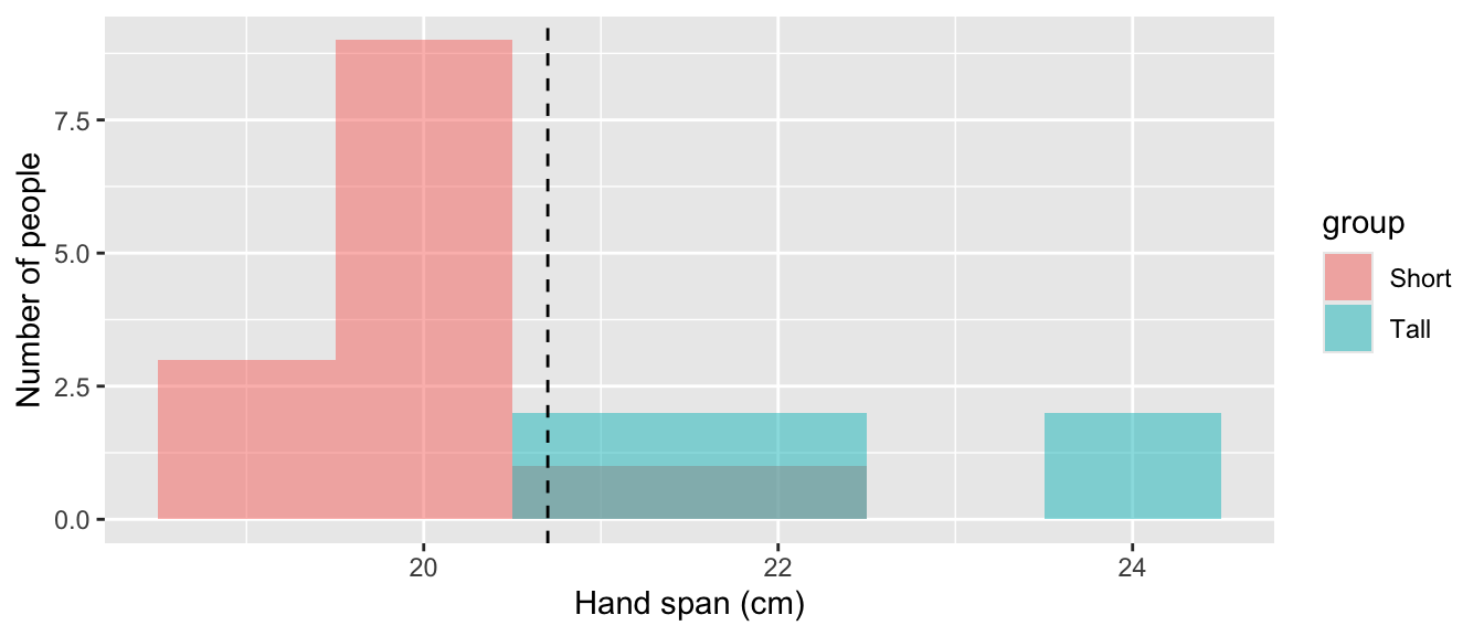
Working as a team on GitHub, and R practice

Due date

This lab is due today, by the end of class. Submit one PDF per group on Gradescope, with every member added to the submission. Your team’s repo on GitHub must show at least one commit from every member.

Introduction

Until now, every repo you have used was made for you, and only you pushed to it. Today your group makes its own repo, and four people work in the same file. You will clone, pull, push, and on purpose create a merge conflict and resolve it.

Then you will practice some R on a small made-up frequency table, taking turns in the shared file:

what a row of a frequency table means, and a mean over the people rather than the rows;
turning the table into one row per person, and a histogram colored by group;
what one overall mean gets wrong for each group;
scoring prediction rules by their sum of squared errors.

Each step builds on the tidyverse and ggplot2 tools from Labs 04 and 05, and explains anything new.

Learning goals

In this lab, you will…

create a GitHub repo, add collaborators, and have everyone clone it;
take turns pulling, editing, committing, and pushing in one shared file;
recognize a merge conflict, read its markers, and resolve it;
compute a mean from a frequency table, and explain why the counts matter;
find what one overall average gets wrong for each group, and compare rules by their squared errors;
read AI-written code line by line, and check it against a result you already know;
state what the course AI policy allows for code and for writing.

Roles and team name

Sit with your project group. Number yourselves Member 1 to 4. In a group of three, Member 2 also does Member 4’s steps.

Choose a team name — short, lowercase, no spaces (for example team-quetelet). Your repo will be called lab-06- followed by that name, for example lab-06-team-quetelet.

One typist, everyone watching

Each step names who does it, but everyone watches. When it is someone else’s step, gather round their laptop and watch their screen as they go: where they click, what they type, what GitHub or RStudio shows back. Say so if something looks different from these instructions. By the end of the lab, each of you should be able to do every step on your own, not only the ones you typed.

Only the member named in a step types in lab-06.qmd, commits, and pushes. Everyone else keeps their hands off their own copy of the file until it is their turn. Pull before you start typing.

Part 1 — Set up the team repo

Every repo you have used so far was created for you. Today Member 1 creates one in their own GitHub account and invites the rest of the group, everyone accepts, and Member 2 adds a .gitignore, all before anyone clones. Do the steps in order: each one needs the one before it. Everyone watches each step on the screen of the person doing it.

1.2 · Member 1: create the repo

Everyone else: watch Member 1’s screen.

Sign in at https://github.com. Click + at the top right, then New repository. (You can also go straight to https://github.com/new.)

Fill in the Create a new repository page:

Field	What to choose
Owner	Your own username. Not `statistical-history`: students cannot create repos there.
Repository name	`lab-06-` plus your team name, for example `lab-06-team-quetelet`. A green check means the name is free.
Description	Leave blank.
Visibility	Private. Only people you invite will see it.
Add README	Turn it on (on some screens it is a box to tick, Add a README file).
.gitignore and license	Leave them as No .gitignore and No license. Member 2 adds your own `.gitignore` in 1.5.

Click Create repository. You land on the repo’s page, which lists README.md. Its address is https://github.com/YOUR-USERNAME/lab-06-TEAM-NAME. Copy it from the browser’s address bar: your teammates need it in 1.4.

1.3 · Member 1: invite your teammates and Kat

Everyone else: watch Member 1’s screen.

On the repo page, click the Settings tab (the gear, at the right of the row of tabs that starts with Code). On a narrow window it may be under the ⋯ menu.
In the left sidebar, under Access, click Collaborators. GitHub may ask you to confirm your password or a two-factor code first.
Click Add people. Type a teammate’s username or email, pick the right person from the list (check the picture), and click Add … to this repository.
Repeat for every teammate, and for KatHusar.

Each person now appears in the list with Pending invite. Send your teammates the repo address you copied in 1.2.

This step stays with Member 1: only a repo’s owner can invite people to it.

1.4 · Members 2–4: accept the invitation

Each of you accepts on your own laptop. Use whichever of these is quickest:

Open the repo address Member 1 sent you with /invitations on the end, for example https://github.com/MEMBER-1-USERNAME/lab-06-team-quetelet/invitations, and click Accept invitation.
Open the email from GitHub (“… invited you to collaborate”), click View invitation, then Accept invitation.
Go to https://github.com/notifications and open the invitation there.

Then open the repo address. You should see README.md. If you see 404 — page not found, you have not accepted yet, or you are signed in to a different GitHub account: a private repo looks as if it does not exist to anyone who is not a collaborator. You cannot clone or push until you accept.

Member 1: reload Settings → Collaborators. Every teammate should now be listed without “Pending invite”. KatHusar may stay pending until Kat accepts during class; that is expected, so carry on.

1.5 · Member 2: add a `.gitignore`

Everyone else: watch Member 2’s screen. Member 2 can do this because accepting the invitation in 1.4 gave them permission to change the repo.

A .gitignore tells Git which files to leave out of the repo. Without it, each person’s RStudio project files get committed, and the first teammate to pull hits an error. It has to be there before anyone clones.

On the repo page, click Add file → Create new file.
In the name box, type .gitignore, with the leading dot.

In the large box below, paste:

.quarto/
*_files/
*.typ
.Rproj.user/
*.Rproj
.Rhistory
.RData
.Ruserdata

Click Commit changes…, then Commit changes again in the box that opens.

Everyone: reload the repo page. It should now list two files, .gitignore and README.md, and the commit should show Member 2’s name.

1.6 · Everyone: one Git setting

Open the Terminal tab in RStudio (next to Console) and run this once:

git config --global pull.rebase false

It tells Git how to combine your work with your teammates’ when you pull. Without it, the first pull after a teammate’s push can stop with a message about divergent branches.

1.7 · Everyone: clone

Exactly as in Lab 01: green Code button → SSH → copy → in RStudio File → New Project → Version Control → Git → paste → Create Project. You should see .gitignore and README.md in the Files pane.

1.8 · Member 3: create the shared document

Everyone else: watch Member 3’s screen.

File → New File → Quarto Document… → Create Empty Document. Paste the block below, fill in the team name and every member’s name, and save it as lab-06.qmd. Render it, then in the Git pane stage lab-06.qmd and lab-06.pdf, commit with a message like “Start lab-06 with team names”, and push.

---
title: "Lab 06: One repo, four people"
subtitle: "Team: ___"
author:
  - "___"
  - "___"
  - "___"
  - "___"
date: today
format: pdf
execute:
  error: true
  warning: true
  message: false
---

**Team motto:** to be decided.

# Part 2 — R practice

# Part 3 — AI and the course policy

Everyone else: pull

Members 1, 2, and 4: click Pull in the Git pane. lab-06.qmd and the PDF appear, with your names in them.

1.9 · Members 3 and 4: make a conflict, then fix it

A merge conflict happens when two people change the same lines and Git cannot tell which version to keep. You will make one on purpose. From step 4 on, everyone watches Member 4’s screen: that is where the conflict appears.

Everyone pulls, so all four copies match.
Members 3 and 4, at the same time and without pulling again: each replace to be decided. in the Team motto line with a different motto. Save, then commit (do not push yet).
Member 3 pushes. It works.
Member 4 pushes. It is rejected: GitHub has a commit that Member 4 does not have yet.
Member 4 pulls. Git cannot combine the two motto lines, so it leaves both in lab-06.qmd, between markers:
```
<<<<<<< HEAD
**Team motto:** Member 4's motto
=======
**Team motto:** Member 3's motto
>>>>>>> 3f9c2a1...
```
The part above ======= is Member 4’s; the part below is what came from GitHub.
As a group, choose the final motto (or combine them). Member 4 edits the file so that one motto line remains and all three marker lines are gone, saves, renders, stages the files, commits (“Resolve motto conflict”), and pushes.

Before Part 2: everyone pulls

Members 1, 2, and 3: pull, so all four copies have the final motto. Member 1 starts 2.1 only after pulling.

Avoiding conflicts

Pull before you start. One typist at a time. Commit and push as soon as your step is done. Conflicts are not errors — they are Git asking a person to decide.

Part 2 — R practice

The data

These numbers are made up for practice. Twenty people from two towns, North and South, were classed as Short or Tall, and each person’s hand span was recorded to the nearest centimeter. The table is in frequency format: each row is a combination of town, height group, and span, with the number of people who had it.

Town	Height group	Hand span (cm)	Number of people
North	Short	19	2
North	Short	20	6
North	Short	22	1
North	Tall	24	1
South	Short	19	1
South	Short	20	3
South	Short	21	1
South	Tall	21	2
South	Tall	22	2
South	Tall	24	1

How the turns work

There are four steps, one for each member. In each step:

Read “What you need” together. It points back to tools you used in Labs 04 and 05 and explains anything new.
The member named in the step pulls, then pastes the copy block at the end of lab-06.qmd, under Part 2.
Everyone works out the blanks together. Members who are not typing should try the code in their own Console (after pulling, use Run → Run All so the earlier objects exist). Typing in the Console does not change the file, so it cannot cause a conflict.
The typist replaces every ___, runs the chunk, and compares the output with What you should see. If it does not match, fix it before going on.
The group answers the step’s Questions under Your answers: in the document.
Hand over (the box at the end of each step): the typist renders, commits, and pushes while everyone watches their screen; then everyone else pulls before the next member starts.

error: true is on, so a chunk with a mistake still renders and shows its error. Fix it anyway: each step uses objects from the steps before.

2.1 · Member 1: what a row means

What you need. In Lab 04 you met the tip always ask what a row means. In urn_color, one row was an urn-and-color combination and its n column said how many balls it stood for, so sum(n) counted balls while n() counted rows. spans is the same kind of table: one row is a town, height group, and span, and count says how many people share it.

That matters for the average. Six people in North have a span of 20, so an average over the people should count 20 six times. Multiply each span by its count, add those up, and divide by the number of people:

\[\text{mean per person} = \frac{\text{sum of (count} \times \text{span)}}{\text{sum of count}}.\]

mean(span) instead counts each row once.

Questions.

What do rows and people each count?
Which mean describes the people, and why is mean_of_rows larger?

## 2.1 What a row means

```{r}
#| label: setup
library(tidyverse)
```

```{r}
#| label: spans
spans <- tibble(
  town  = c("North", "North", "North", "North", "South",
            "South", "South", "South", "South", "South"),
  group = c("Short", "Short", "Short", "Tall", "Short",
            "Short", "Short", "Tall", "Tall", "Tall"),
  span  = c(19, 20, 22, 24, 19, 20, 21, 21, 22, 24),
  count = c(2, 6, 1, 1, 1, 3, 1, 2, 2, 1))
spans
```

```{r}
#| label: average
span_summary <- spans |>
  summarize(rows = n(), people = sum(___),
            mean_of_rows = mean(span),
            mean_per_person = sum(___ * ___) / sum(count))
span_summary
span_mean <- span_summary$mean_per_person
```

**Your answers:**

What you should see: rows 10, people 20, mean_of_rows 21.2, and mean_per_person 20.7.

Hand over to Member 2

Member 1: render, then commit (message: 2.1) and push.
Members 2, 3, and 4: pull. Member 2 starts 2.2 only after pulling.

2.2 · Member 2: one row per person, and a histogram

What you need. Two new functions, and one you know.

uncount(count) is the reverse of count(): it repeats each row as many times as its count and drops the count column. The result has one row per person, which is what ggplot() expects.
geom_histogram(binwidth = 1) draws one bar per centimeter, its height the number of people. Look it up on the ggplot2 cheatsheet if you like.
Putting fill = group inside aes() colors each bar by height group and stacks the two colors. As in Lab 05, something looked up per row goes inside aes().
geom_vline() from Lab 05 draws a vertical line, here at the mean.

Questions.

Does the mean of people match span_mean from 2.1? Why?
Describe the histogram: where is its center, and how spread out is it?
Where do the Short people sit relative to the dashed line, and where do the Tall people sit?

## 2.2 One row per person, and a histogram

```{r}
#| label: people
people <- spans |>
  uncount(___)
people |>
  summarize(people = n(), mean_span = mean(span))
```

```{r}
#| label: span-histogram
ggplot(people, aes(x = ___, fill = ___)) +
  geom_histogram(binwidth = 1) +
  geom_vline(xintercept = ___, linetype = "dashed") +
  labs(x = "___", y = "Number of people",
       title = "Hand spans, both towns")
```

**Your answers:**

What you should see: 20 people with a mean of 20.7. Bars at 19 to 24 with heights 3, 9, 3, 3, 0, 2 (no one at 23), the Short people mostly at 19–20 and the Tall people at 21, 22, and 24, and a dashed line at 20.7.

Side note: other ways to show two groups (read only, nothing to run)

The histogram you made is stacked: within each bar, the Tall people sit on top of the Short people, so every bar is exactly as tall as in a histogram of everyone together. The outline of the pooled histogram does not change; the colors only show who is inside each bar.

If you wanted to see each group’s own histogram instead, there are two common options.

Overlapping. position = "identity" starts both groups’ bars at zero, one in front of the other, and alpha makes them see-through. Where the groups share a span (21 and 22 here), the colors blend:

ggplot(people, aes(x = span, fill = group)) +
  geom_histogram(binwidth = 1, position = "identity", alpha = 0.5) +
  geom_vline(xintercept = span_mean, linetype = "dashed") +
  labs(x = "Hand span (cm)", y = "Number of people")

Side by side. facet_wrap(~ group, ncol = 1) draws one small histogram per group, stacked vertically on the same horizontal axis:

ggplot(people, aes(x = span, fill = group)) +
  geom_histogram(binwidth = 1) +
  geom_vline(xintercept = span_mean, linetype = "dashed") +
  facet_wrap(~ group, ncol = 1) +
  labs(x = "Hand span (cm)", y = "Number of people")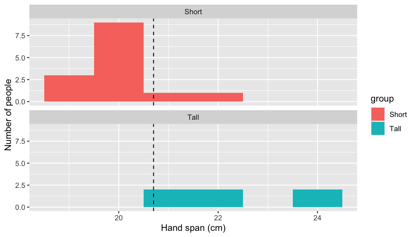

Both make the groups easier to compare with each other, but neither shows the pooled histogram. The stacked version shows both at once, which is why we used it.

Hand over to Member 3

Member 2: render, then commit (message: 2.2) and push.
Members 1, 3, and 4: pull. Member 3 starts 2.3 only after pulling.

2.3 · Member 3: what one average hides

What you need. In Lab 05, a guess’s error for each reading was the observed value minus the guess. Here the guess is span_mean for everyone. A positive error means the guess was too low for that person; a negative one, too high.

This step makes two tables:

Table	Group by	One row for each
First	`group`	height group: Short, Tall
Second	`town` and `group`	town-and-height-group combination: North Short, North Tall, South Short, South Tall

In the first, mutate() adds each person’s error as a new column, then group_by() and summarize() (Lab 04) average it within each height group. The template fills in most of it.

The second you write yourself, starting from people |>. Group by two columns at once, as in Lab 04’s group_by(urn, color), then summarize the number of people (people) and their mean span (mean_span) in each combination.

Questions.

In the first table, which height group does span_mean predict too high, and which too low? How can you tell from mean_error?
In the second table, which mean is based on only one person?
Do we need mutate() in the second table? Why or why not?

## 2.3 What one average hides

```{r}
#| label: group-means
# First table: one row per height group
people |>
  mutate(error = span - ___) |>
  group_by(___) |>
  summarize(people = n(), mean_span = mean(span),
            mean_error = mean(___), .groups = "drop")

# Second table: one row per town and height group.
# Write the rest of the pipeline yourself.
people |>
```

**Your answers:**

What you should see: Short: 14 people, mean 20, mean error −0.70. Tall: 6 people, mean 22.33, mean error +1.63. Then North Short 20, North Tall 24, South Short 20, South Tall 22.

Hand over to Member 4

Member 3: render, then commit (message: 2.3) and push.
Members 1, 2, and 4: pull. Member 4 starts 2.4 only after pulling.

2.4 · Member 4: one number for each rule

What you need. In Lab 05 you scored a guess with the sum of squared errors: square each error and add them up. Here we score three rules for predicting a person’s span:

one overall mean for everyone;
the mean of their height group;
the mean of their town-and-height-group combination.

To give every person their own group’s mean, use group_by() and then mutate() instead of summarize(). mutate() computes within each group but keeps every row, so each person gets their group’s mean next to their span. ungroup() afterwards stops later steps working within groups, like .groups = "drop" in Lab 04.

Questions.

Which rule has the smallest sum of squared errors?
Rule 3 predicts North’s one Tall person exactly. Would you bet that the next Tall person from North also has a 24 cm span?
What is the difference between fitting the people you have and predicting new people?

## 2.4 One number for each rule

```{r}
#| label: three-rules
people |>
  group_by(group) |>
  mutate(group_mean = mean(span)) |>
  group_by(town, group) |>
  mutate(cell_mean = mean(___)) |>
  ungroup() |>
  summarize(rule_1 = sum((span - span_mean)^2),
            rule_2 = sum((span - ___)^2),
            rule_3 = sum((span - ___)^2))
```

**Your answers:**

What you should see: rule_1 40.2, rule_2 17.3, rule_3 14.

Hand over to Member 1

Member 4: render, then commit (message: 2.4) and push.
Members 1, 2, and 3: pull. Member 1 starts Part 3 only after pulling.

Part 3 — AI writes code; you read it

3.1 · Member 1: ask for code

The course syllabus lets you use AI to ask coding questions or debug code. First make a genuine attempt yourself — you already have: you found these means in R in 2.3. Do not copy and paste a prompt from these instructions; formulate your own question.

As a group, write your own request, in your own words, asking an AI tool of your choice for R code that finds the mean span for each town and height group from spans, counting each person once. Describe the data frame and its columns so the tool knows what it is working with.

Paste under Part 3 in lab-06.qmd, fill in the request and the record line, and paste the AI’s code into the chunk unchanged:

## 3.1 The AI's code

Our request, in our own words: ___

Tool and model: ___. Date: ___. Link to the full conversation: ___.

```{r}
#| label: ai-code
# Paste the AI's code here, unchanged.
```

Do not run it yet.

Hand over to Member 2

Member 1: save, then commit (message: 3.1) and push without rendering: rendering would run the AI’s code before you have read it.
Members 2, 3, and 4: pull. Member 2 starts 3.2 only after pulling.

3.2 · Member 2: read it before running it

Questions.

Go through the AI’s code line by line as a group. What does each line do, in your own words?
Before running it: what four numbers should it print? (You already know them from 2.3.)
Now render. Does it print 20, 24, 20, and 22? If not, which line went wrong, and why?

A common mistake is averaging the rows of spans instead of the people; that gives 20.33 for North Short and 22.33 for South Tall.

## 3.2 Reading the AI's code

**What each line does:**

**What we predicted it would print:**

**What it printed, and why:**

Hand over to Member 3

Member 2: render, then commit (message: 3.2) and push.
Members 1, 3, and 4: pull. Member 3 starts 3.3 only after pulling.

3.3 · Member 3: what does the course allow?

Open the Generative artificial intelligence section of the syllabus. As a group, answer in your own words — not with AI.

Questions.

Are you allowed to use AI in this course? Under what two principles?
May you use AI to help with code? What must you do first, and what must you be able to do afterwards?
May you use AI to write the narrative you submit?
What must you record when AI materially informs your work?
Why did 3.1 ask you to write your own request rather than copy one? How could you use AI on the code for your homework within these rules?

## 3.3 Course policy

**Your answers:**

Hand over to Member 4

Member 3: render, then commit (message: 3.3) and push.
Members 1, 2, and 4: pull. Member 4 does the wrap-up only after pulling.

Wrap-up

Member 4: final render, push, and submit

Pull, render, and check the PDF: team name, every member’s name, the motto, every step from 2.1 to 3.3 with its answers.
Commit and push, so the Git pane is empty for everyone after they pull.
Upload the PDF to Gradescope once, then add every group member to the submission.
On GitHub, open the repo’s commits page and check that each member has at least one commit.

Exit ticket (on paper, with your name):

Muddiest point.
One thing you learned today.
Favorite fall food.

If you finished early

Neither of these is graded, and you are not behind if you never reach them. Any member may paste one at the end of lab-06.qmd: pull first, then render, commit, and push, and tell your group so they pull too.

Extra 1: cumulative fractions and `qnorm()`

For each span, \(F\) is the fraction of people with that span or less: a running total of people, from Lab 02’s cumsum(), divided by everyone. In HW 02 you used pnorm(z), the fraction of the standard normal curve to the left of the cutoff z; for example pnorm(0) is 0.5. The new function qnorm(p) goes the other way: give it a fraction, and it returns the cutoff. qnorm(0.5) is 0 and qnorm(0.975) is about 1.96.

Question. What does qnorm() give for the last row, and why?

## Extra 1: cumulative fractions

```{r}
#| label: cumulative
spans |>
  group_by(span) |>
  summarize(people = sum(count), .groups = "drop") |>
  mutate(F = cumsum(___) / sum(people),
         z = qnorm(___))
```

**Your answer:**

What you should see: \(F\) = 0.15, 0.60, 0.75, 0.90, 1 and \(z\) = −1.04, 0.25, 0.67, 1.28, Inf.

Extra 2: a normal curve on the histogram

To draw a normal curve over a histogram, both must be on the same scale. aes(y = after_stat(density)) rescales the bars so their total area is 1, like the area under a normal curve, and stat_function() draws the curve dnorm() with the mean and standard deviation you give it. The standard deviation here divides by the number of people.

Question. Does the normal curve describe these 20 spans well? Where does it miss?

## Extra 2: a normal curve on the histogram

```{r}
#| label: normal-curve
span_sd <- sqrt(sum((people$span - span_mean)^2) / nrow(people))
ggplot(people, aes(x = span)) +
  geom_histogram(aes(y = after_stat(density)), binwidth = 1) +
  stat_function(fun = dnorm,
                args = list(mean = ___, sd = ___)) +
  labs(x = "Hand span (cm)", y = "Density")
```

**Your answer:**

What you should see: span_sd is about 1.42; the curve peaks near 20.7, below the tall bar at 20.

Introduction

Learning goals

Roles and team name

Part 1 — Set up the team repo

1.1 · Everyone: share your GitHub usernames

1.2 · Member 1: create the repo

1.3 · Member 1: invite your teammates and Kat

1.4 · Members 2–4: accept the invitation

1.5 · Member 2: add a .gitignore

1.6 · Everyone: one Git setting

1.7 · Everyone: clone

1.8 · Member 3: create the shared document

1.9 · Members 3 and 4: make a conflict, then fix it

Part 2 — R practice

The data

How the turns work

2.1 · Member 1: what a row means

2.2 · Member 2: one row per person, and a histogram

2.3 · Member 3: what one average hides

2.4 · Member 4: one number for each rule

Part 3 — AI writes code; you read it

3.1 · Member 1: ask for code

3.2 · Member 2: read it before running it

3.3 · Member 3: what does the course allow?

Wrap-up

If you finished early

Extra 1: cumulative fractions and qnorm()

Extra 2: a normal curve on the histogram

1.5 · Member 2: add a `.gitignore`

Extra 1: cumulative fractions and `qnorm()`