Skip to main content

119 STA 119FS Statistics as a Way of Thinking

Course Questions Calendar

Materials ▾

• Syllabus
• Materials overview
• Assignments
• Historic Timeline

Lab 01: Mayer’s method of averages

ImportantDue date

This lab is due today, by the end of class. To be considered on time:

• lab-01.qmd committed and pushed to your GitHub repo before the exit ticket
• That same document, rendered to PDF, submitted on Gradescope

Introduction

In 1750 Tobias Mayer wanted to measure the libration of the moon — the slight wobble that lets us see a bit around its edge. He took 27 observations, and each one gave him an equation in the same 3 unknowns.

27 equations, 3 unknowns. More information than he needed. That sounds like good news.

It wasn’t, and here’s why: the 27 equations contradict each other. There is no set of three numbers that satisfies all 27. There isn’t even a set that satisfies four of them. Every observation has a little error in it, so every equation is slightly wrong, and they’re all slightly wrong in different directions.

At the same time, Leonhard Euler — a far greater mathematician than Mayer — had 75 equations in 8 unknowns for the orbits of Jupiter and Saturn. He gave up. He didn’t believe you were allowed to combine measurements that disagreed; he thought errors would pile up rather than cancel.

Mayer wasn’t a better mathematician. He just wasn’t afraid of the data. Today you find out what he did.

Learning goals

By the end of this lab you will be able to…

• call functions, pass arguments by position and by name, and keep what they return.
• pull a column out of a data frame with $, and hand it to a function.
• tell a base R function from one written for this course, and read a course-written one when there is no help page to open.
• explain why 27 equations in 3 unknowns have no exact answer, and why base R will not even attempt one.
• reproduce Mayer’s grouped-sum method and judge whether his grouping rule matters.
• commit and push your work to GitHub.

---

Part 1 — together

Getting your repo

Note

The rest of Part 1 is not group work and nothing in it is graded on being right. Laptops open, follow along, and stop me the second a step doesn’t do on your screen what it does on mine. Everything after this depends on this part working.

1 · Find the repo. Go to the statistical-history organization on GitHub and click the repo whose name starts with lab-01. This is your first private repo for this course — not the public one from lab-00.

2 · Copy the SSH address. Green Code button. Make sure SSH is selected — the label should read Clone with SSH and the address should start with git@github.com:, not https://. Copy it.

3 · Make it a project. In RStudio: File → New Project → Version Control → Git. Paste the address into Repository URL, leave the directory name as it fills itself in, click Create Project. RStudio clones the repo and opens it. You should see lab-01.qmd, a data/ folder, and lab-01-helpers.R in the Files pane.

4 · Put your name in it. Open lab-01.qmd and look at the very top, between the two --- lines. That block is the YAML — it holds the document’s title, author, and formatting options, not its content. Change the subtitle so it has your group’s card and put your names in author.

5 · Render it. The Render button at the top of the Source pane. A PDF appears — lab-01.pdf, in the same folder. That’s the file you were just looking at, turned into something readable, and it is exactly the file you’ll hand in. Render often; it’s how you find out early that a chunk is broken.

6 · Commit and push. Git pane (top right, its own tab, next to Environment). Your changed lab-01.qmd is listed and lab-01.pdf is added. Tick the box to stage it, write a message — “Added our names”, not “updates” — click Commit, then click Push.

ImportantStep 6 is the one that matters — verify it

Open your repo’s page on GitHub and refresh. You should see your commit message and your own names sitting there.

TipYour repo isn’t in the organization?

Most likely your entry survey response is still processing, or the GitHub username you gave doesn’t match your actual account. Say so now — don’t work around it and end up with nothing to push.

TipStep 2 gave you an https:// address?

Switch it to SSH before you clone. An https:// address asks for a password on every single push and will not accept your GitHub password.

Where the text goes and where the code goes

Now that everyone has the file open — this is what you’re looking at.

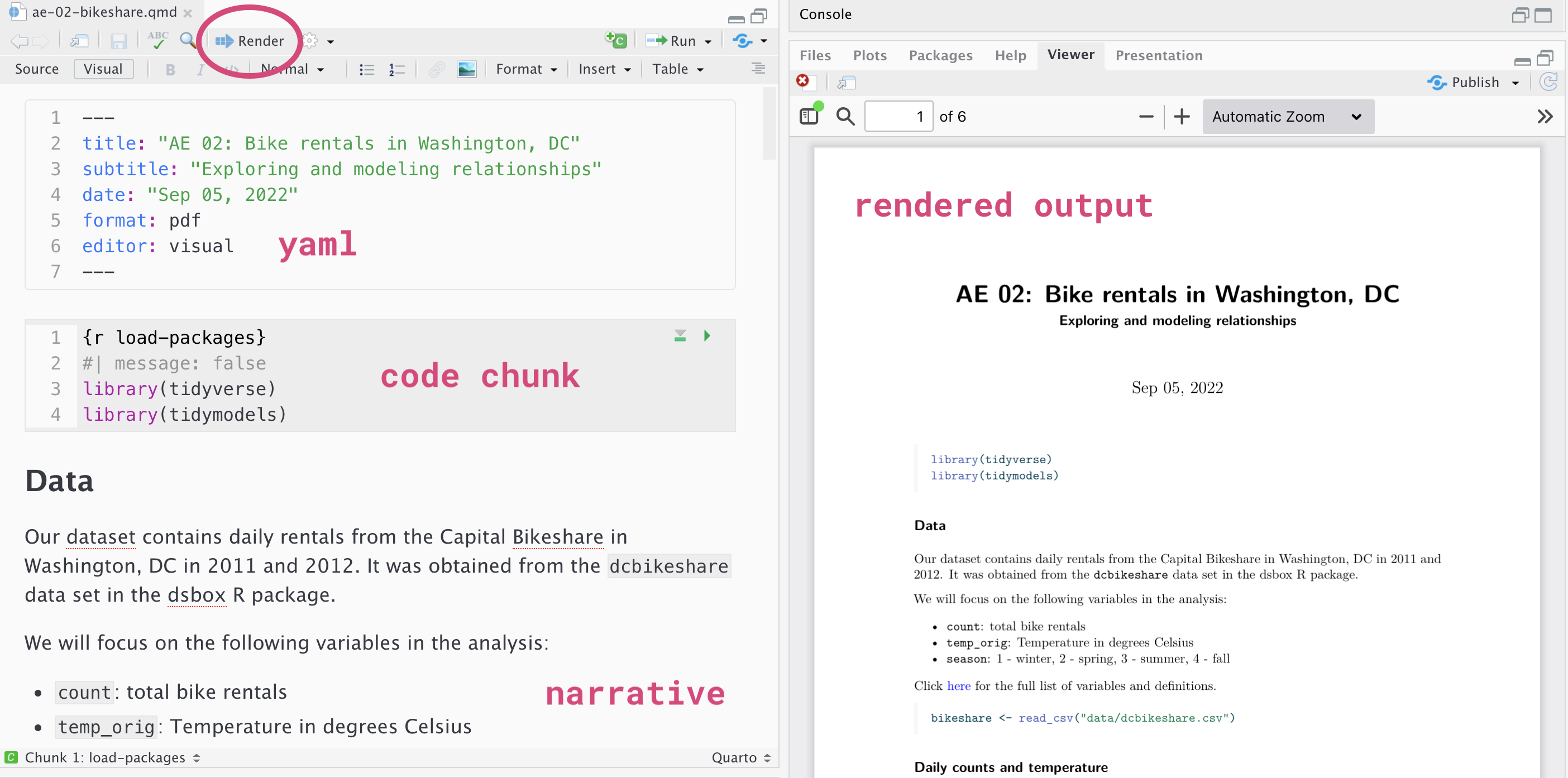
A .qmd file has exactly three kinds of thing in it:

Part	What it is	Where you type
YAML	The block at the top between --- lines. Title, author, options	Only when a step tells you to
Text	Ordinary writing. Answers, reasoning, anything in prose	Anywhere outside a chunk
Code chunks	The grey blocks that start ```{r} and end ```. R runs what’s inside	Only inside the grey

Text typed inside a chunk is an error. Code typed outside a chunk is just words. That is the single most common thing to go wrong today, and it looks like the file is broken when it isn’t.

And here is the window it all lives in:

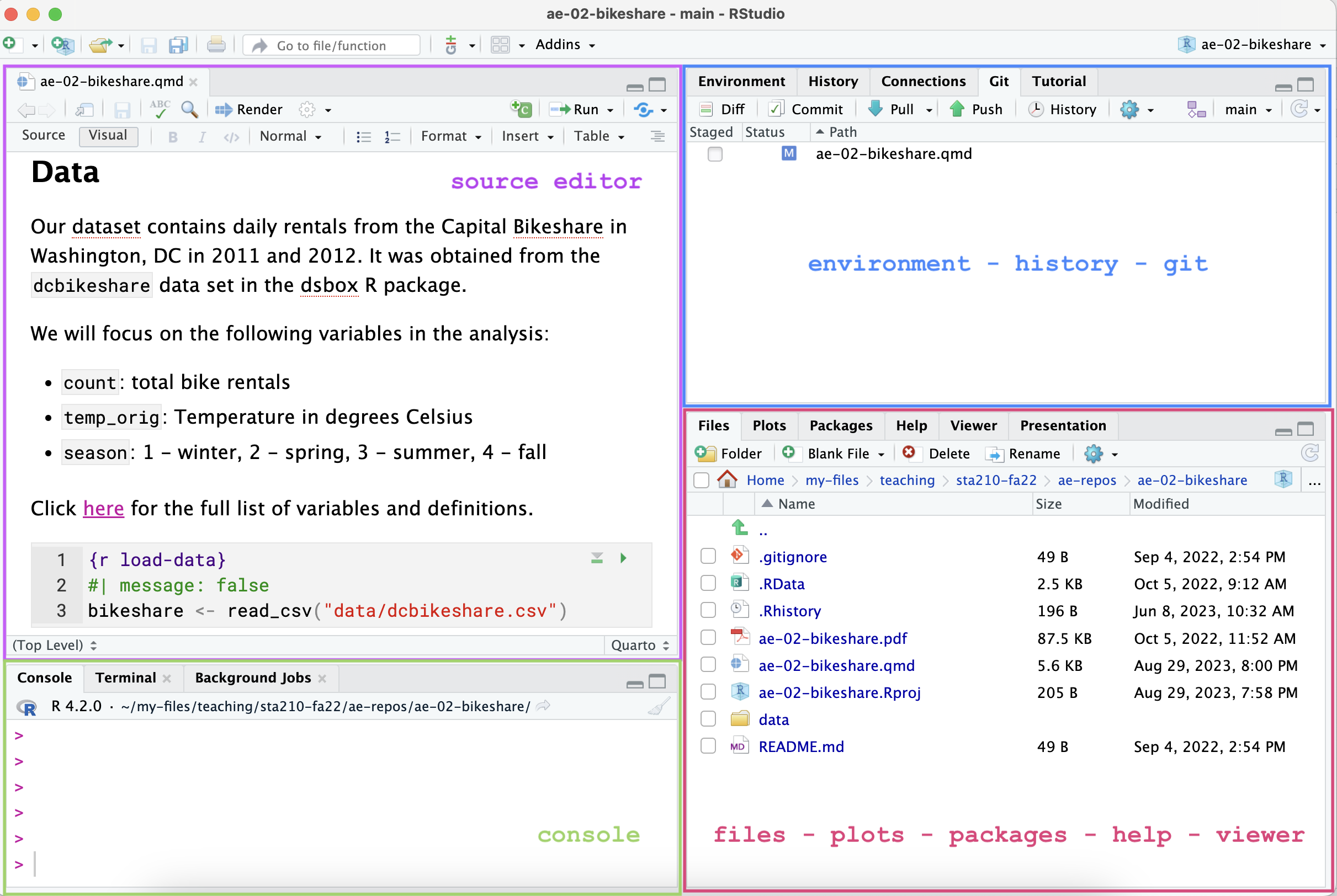
• Source (top left) — your open files, like lab-01.qmd. Where you write.
• Console (bottom left) — where code actually runs. You can type here too, but anything you want to keep goes in lab-01.qmd instead.
• Environment / History (top right) — everything you’ve made so far this session. The Git pane is a tab here.
• Files / Plots / Packages / Help (bottom right) — your project’s files, your plots, and R’s documentation.

Committing, for the rest of the day

You just did it once. Two things worth knowing for the next hour:

• Render updates the pdf. Commit saves a snapshot on your own machine. Push sends it to GitHub. You need to do all three.
• Before you stage a file, click it and click Diff. That shows what changed since the last commit — red is gone, green is new. It’s how you catch an edit you didn’t mean.

You’ll be told to commit at several points today. With time, you’ll determine best times to commit and push on your own.

Part 2 — Your first R, also together

The assignment arrow

total <- 6

Nothing printed. <- is the assignment arrow: it says take the thing on the right and store it under the name on the left. It stores instead of showing. To see what’s in something, type its name on its own line:

total

[1] 6

Objects live in your R session, not inside the chunk that made them — so every chunk below can use total now, and so can the console. This is also why chunk order matters: a chunk that uses total fails if you run it before the chunk that creates total.

Putting several things together: c()

rows <- c(1, 2, 3)
rows

[1] 1 2 3

c() is short for combine. It takes several values of the same type and makes them one vector. So c(1, 2, 3) is one thing holding three numbers — not three separate things. You’ll hand vectors to functions constantly, starting in about ten minutes.

You just called your first function — c() — and nearly everything you do in R for the rest of the semester is a function call too. Next week’s homework leans on this heavily, so here is what a call actually is before you meet twenty more of them.

What a call is made of

sum(c(1, 2, 3))

[1] 6

• sum is the function’s name.
• () are what make it run. Typing sum on its own doesn’t add anything up — it just shows you the function itself. The parentheses are the “do it now” part.
• c(1, 2, 3) is an argument — the input you’re handing over. Some functions take none, some take several separated by commas.
  • c() is itself a function, and one you’ll use constantly. Its name is short for combine (sometimes said as concatenate). It takes several elements of the same type and puts them together into a single vector. So c(1, 2, 3) is one vector holding three numbers — not three separate arguments to sum().
• The function hands something back. Here that’s the number 6.

What comes back vanishes unless you catch it, so most of the time you assign it a name:

total_sum <- sum(c(1, 2, 3))

Arguments can be given by position or by name. These two are the same call:

round(3.14159, 2)

[1] 3.14

round(3.14159, digits = 2)

[1] 3.14

Naming them is slower to type and much easier to read. When a function takes more than two arguments, name them.

Three kinds of function, and only one of them has a help page

Kind	Examples	Where it comes from	Does ?name work?
Base R	sum(), solve(), lm(), read.csv()	Built into R. Always available	Yes — try ?sum
From a package	none today	You install.packages() once, then library() each session	Yes, once loaded
Written for this course	solve_rows(), and a pile more next week	A .R file we hand you. You run source() on it	No. It exists nowhere else

That third row is the we will mostly use today and in homework 1. They are not magic and they are not advanced — each one is a few lines of ordinary R that you could have written, packaged up so that a whole procedure fits in one line.

The catch: ?solve_rows won’t work, and searching the internet for it won’t either. If you want to know what one does, open the file and read it — which is exactly what you’ll do in Part 4.

Part 3 — The data

Loading the data

practice_df <- read.csv("data/practice_equations.csv")
dim(practice_df)

[1] 27  5

head(practice_df)

  obs a  b  c  rhs
1   1 1  5 -4 1403
2   2 1  5  5 1136
3   3 1 -3 -1  671
4   4 1  1  5  827
5   5 1  0 -3  925
6   6 1 -1  4  656

read.csv() reads the file; <- stores it as practice_df; dim() says how big it is and head() shows the top of it. 27 rows and 5 columns.

What one row actually says

Each row is one equation. Its four number columns are things you measured, and they sit in front of three unknowns you are trying to find:

\[a_i \times x_1 \;+\; b_i \times x_2 \;+\; c_i \times x_3 \;=\; \texttt{rhs}_i\]

The subscript \(i\) is the row number: every row brings its own \(a_i\), \(b_i\), \(c_i\) and \(\texttt{rhs}_i\). The unknowns carry no subscript, on purpose — \(x_1\), \(x_2\) and \(x_3\) are the same three numbers in all 27 rows.

So take row 1, which reads 1, 1, 5, -4, 1403:

obs	a	b	c	rhs
1	1	5	−4	1403

and that row is this equation:

\[1 \times x_1 \;+\; 5 \times x_2 \;-\; 4 \times x_3 \;=\; 1403\]

One equation, three unknowns — not solvable on its own. Row 2 is a different equation about the same three numbers. So is row 27.

ImportantWhat you are actually holding

27 equations. 3 unknowns. More equations than unknowns, and the 27 equations contradict each other. Every observation carries a little error, so every equation is slightly wrong, and they’re all wrong in different directions. There is no set of three numbers that satisfies all 27 — there isn’t even a set that satisfies four of them.

ImportantThese numbers are made up.

practice_equations.csv is not Mayer’s data. We built it. Same shape as his table (27 equations, 3 unknowns, a constant term, errors that stop any three numbers from satisfying all 27). Homework 1 uses Mayer’s real table.

---

Getting one column out: $

practice_df$rhs

 [1] 1403 1136  671  827  925  656  426 1104  320 1249  402 1371  884 1043  317
[16]  533 1303  813  483  921 1125  505 1188  788  918 1162  867

sum(practice_df$rhs)

[1] 23340

$ pulls one column out of a data frame by name, and what comes back is a vector — the same kind of thing c(1, 2, 3) made earlier.

Next week’s homework asks you for sum(group_I$constant_arcminutes) — a data frame, one column pulled out of it by name, and those nine numbers added up.

Part 4 — Lab 01’s helpers

Try them

Four of them, in lab-01-helpers.R. Load the file, then run the first three.

source("lab-01-helpers.R")

source() is base R. It means “run every line of that file” — which, for a file that contains only function definitions, means all four functions now exist and you can call them. Nothing appears when it works. If you later get could not find function "solve_rows", this line is what didn’t run.

check_equations(practice_df)

Looks right: 27 equations, 3 unknowns, no missing values.

This one checks the file you loaded is the one this lab expects. No news is good news — if something were wrong it would stop and tell you.

show_equation(practice_df, 1)

[1] "Equation 1:  1 * x1  + 5 * x2  - 4 * x3  =  1403"

show_equation(practice_df, 4)

[1] "Equation 4:  1 * x1  + 1 * x2  + 5 * x3  =  827"

Row 1 of a CSV is not obviously an equation. This writes out the same thing you saw in Part 3 — 1 * x1 + 5 * x2 - 4 * x3 = 1403 — straight from the row. Try a few other row numbers.

NoteR counts from 1

show_equation(practice_df, 1) gives you the first row, and practice_df has 27 rows numbered 1 through 27. If you’ve written Python, Java, C, or JavaScript before, this is the opposite of what you’re used to: those languages start at 0, so their “first” element is number 0 and their last is number n − 1.

R starts at 1 and goes to n, which matches how the rest of the course talks — “equation 1” is practice_df[1, ], and the last one is practice_df[27, ]. Two things that catch people coming from those other languages: practice_df[0, ] isn’t an error, it just hands back an empty result, which is a confusing way to discover you were off by one; and a negative number doesn’t count from the end, it means drop — practice_df[-1, ] is all 27 rows except the first.

solve_rows(practice_df, c(1, 2, 3))

       x1        x2        x3 
882.45833  80.37500 -29.66667 

Three unknowns, from equations 1, 2, and 3 — which is exactly what Exercise 2 is about to have you do by hand.

Reading a function definition

For this lab and Homework 01, all you need to do is call a function and know what it does. Reading the definition is how you find out what it does — so it’s worth learning to read one, even before you write one. Here’s the shape, stripped down:

sum_rows <- function(equations, rows) {   # name <- function(inputs) {
  c(colSums(equations[rows, c("a", "b", "c")]),
    rhs = sum(equations$rhs[rows]))       #   the last value is what comes back
}                                         # }

That is the real sum_rows() from lab-01-helpers.R, minus its two error checks — you’ll call it in Exercise 3.

function(equations, rows) says “this takes two inputs, and inside here I’ll call them equations and rows.” Everything between the braces is the body. Whatever the body’s last line evaluates to is what the function hands back. So sum_rows(practice_df, group1) runs that body with equations set to practice_df and rows set to group1.

Note

Notice the argument is called equations inside the definition but you pass it practice_df. That’s not a mistake. A function names its own inputs; what you hand in keeps its own name outside. These helpers would work on any table shaped like ours, which is why they aren’t named after ours.

R lets you say that last part out loud with return(), and many languages require it. These two definitions behave identically:

add_one <- function(x) {
  x + 1              # last value evaluated, so it's what comes back
}

add_one <- function(x) {
  return(x + 1)      # says the same thing explicitly
}

---

Part 5 — Exercises

Goal: turn 27 contradictory equations into a single, defensible claim about 3 unknown quantities — and understand why that turn was Mayer’s invention, not the arithmetic after it.

1. Predict

In your groups. Agree on an answer, then we vote as a room. Write it in lab-01.qmd before you run anything.

Prediction. You’re about to draw 3 of the 27 equations and solve them exactly. The group next to you draws a different 3. How much will the two answers disagree?

(a) essentially the same three numbers (b) different in size, but pointing the same way (c) far enough apart that even the signs could disagree

2. Draw three equations and solve them

Draw them

Each group draws three numbered slips. Not 1, 2, 3 — whatever you draw. Write the three numbers down; you’ll need them twice.

Solve them

Here’s the shape of it, using rows 1, 2, 3:

solve_rows(practice_df, c(1, 2, 3))

       x1        x2        x3 
882.45833  80.37500 -29.66667 

One call: hand it the table and three row numbers, get back the three unknowns. solve_rows() is one of the course-written functions, so open lab-01-helpers.R and read it.

Inside you’ll find three ordinary lines: pull out those rows, pull out their right-hand side, solve. Now do it with the three equations you drew, using solve_rows().

Put it on the board

Each time, write these on the board and then in lab-01.qmd:

The three equation numbers you drew	so we can see nobody had the same three
The three numbers you got	\(x_1\), \(x_2\), \(x_3\)

Four groups — J, Q, K, A — four rows.

TipNow look at the board — this is the whole of Chapter 1

Check the board against Prediction 1.

Commit and push now: “solved our three equations.” Everyone in your group does this on their own machine — this course has no driver/navigator split, you all type everything.

3. Mayer’s fix

Mayer’s idea: don’t throw 24 equations away. Add them up.

Sort the 27 equations into three groups of nine, add each group together to make one equation, and solve the resulting 3×3.

His rule for how to sort them: put equations in different groups when their measured \(b\) values are as different as possible. Note that this is a rule about the measured numbers, not about the answers — he sorts on a column he can read straight off the table, and chooses his groups before he knows what they’ll give him.

Sorting, and what group1 actually holds

ordered_rows <- order(practice_df$b)

group1 <- ordered_rows[1:9]
group2 <- ordered_rows[10:18]
group3 <- ordered_rows[19:27]

group1

[1]  7  9 16 11 15 22  3 18 19

Importantgroup1 is a list of row numbers — not equations, not answers

order() doesn’t sort the data. It hands back the row numbers, in the order that would sort them — so ordered_rows is all 27 row numbers arranged from the most negative b to the most positive.

ordered_rows[1:9] then takes the first nine of those numbers. So group1 is nine row numbers: it means “the nine equations with the smallest b.” Printing group1 above shows you exactly which nine, and they are not 1 through 9.

Here is the whole maneuver in one picture — 27 equations sorted, cut into three groups of nine, each group added down into a single equation:

Doing it

sum_rows() is the fourth helper in lab-01-helpers.R. It takes the data and some row numbers, adds those rows up column by column, and hands back one equation:

sum_rows(practice_df, group1)

   a    b    c  rhs 
   9  -36    4 4470 

Four numbers: the summed \(a\), \(b\) and \(c\), and the summed right-hand side. That is one equation. Do it three times and stack the results:

M <- data.frame(rbind(sum_rows(practice_df, group1),
           sum_rows(practice_df, group2),
           sum_rows(practice_df, group3)))

answer <-solve_rows(M, c(1:3))
answer

 x1  x2  x3 
870  90 -30 

One answer, from all 27 equations. I’ll put that one on the board next to your four.

4. The modern tool

It’s a one-liner black box you’ll learn about soon in the course. For now the point is only that a third answer exists.

fit <- lm(rhs ~ b + c, data = practice_df)
coef(fit)

(Intercept)           b           c 
  869.68247    90.51027   -28.28532 

All 27 rows, no grouping, no choosing. A different answer again.

It is better than Mayer’s, in a specific sense — but that sense doesn’t exist yet in this book. It gets invented in Chapter 4. Hold the question.

Commit and push: “Mayer’s grouping and lm().”

5. Debrief

You have three kinds of answer in front of you. Look at all three before you say anything.

One — the four answers from three equations each

One draw per group, four sets of three numbers on the board.

• How different are they from each other? Put a number on it if you can — how far apart are the largest and smallest \(x_2\)?
• Every one of those four is exactly correct for the three equations that produced it. So what is it that’s actually wrong?
• Nobody drew badly. Is there a set of three you could have drawn that would have been the right three?

Two — how do they compare to Mayer’s answer?

One solution from all 27 equations.

• Where does it sit relative to the four? In among them? Off to one side?
• If you’d only ever seen your own group’s three-equation answer, would you have had any way to know it was off?

Three — how do they compare to lm()?

• Mayer’s grouped answer and lm() both used all 27 equations. How close are they to each other, compared with how close the four are to each other?

Prediction 1 — settled

You predicted how far apart two groups’ three-equation answers would be. The board is the answer, and it’s sitting right there. Check what your group wrote against it.

What happens next

Four answers is not much to reason from, and you only tried one way of grouping. The homework does both at scale, on Mayer’s real 27 equations:

You did	The homework does
4 answers from three equations each	1,000 of them
1 grouping — Mayer’s own sorted one	1,000 random regroupings, plus a third rule: one equation from each of Mayer’s groups — and the question of whether his sorting rule mattered at all

Part 6 — AI slot

Commit and push: Good moment for the Git pane to go empty.

The governing rule of this course is that you may not submit a line of code you can’t explain. So the genuinely useful thing to ask a model for, today, is not code — it’s an explanation. You’re going to ask for the same explanation twice. The function stays the same both times; the only thing that changes is the prompt.

Open lab-01-helpers.R and find show_equation(). That is the function for both prompts. You’ve already run it — Section 3 — so you know what it produces.

Prompt 1 — the one you’d actually type

Explain this R function.

Prompt 2 — the same question, specified

I’ve never written R and I’m new to coding — assume I know what a variable is and nothing else. Walk through this function step by step. One sentence per step, and name every R function it uses. Then tell me what goes in and what comes out, and what kind of thing each one is — a number, a table, a piece of text, one of them or many. Then invent a small input and trace it through in a table, one row per step, ending at the value the function hands back. No summary, no suggested improvements, and don’t rewrite the code.

Tip

Copy both prompts off this page rather than retyping them, and paste show_equation() underneath each one.

---

Think — on your own

Run both prompts. Read both answers. Don’t talk to anyone yet.

Then write down, in lab-01.qmd, before you discuss it: one thing the second answer told you that the first didn’t. Which part of the prompt helped pin down that part?

Group — the four of you

Share your thoughts with the group. Write down what your group agreed on.

Share — whole class

Important

What did Prompt 2 pin down that Prompt 1 left open?

One from each group.

Prompt 2 isn’t longer for the sake of it, and it isn’t a magic phrase to save and reuse. Every clause in it is a decision the model was going to make either way. Unasked, it makes them for the average person who pastes in code — who is not you.

Render and commit again. Push.

Part 7 — Exit ticket

On paper, handed in as you leave :

1. Muddiest point?
2. One thing you’d want to try in R next.
3. Any plans for the weekend?

Make sure your name is on it as this is how attendance is taken.

---

Submission

Warning

Before you leave, make sure lab-01.qmd is fully committed and pushed. Check your Git pane: it should be empty. If it isn’t, something didn’t push, and that’s the thing to fix before the exit ticket, not after.

You must also submit lab-01.pdf on Gradescope before the deadline for full credit. That’s the file the Render button already made for you — this document renders straight to PDF, so there is no separate export step and nothing to combine. Render once more at the end so the PDF matches your final text.

To submit on Gradescope:

• Click on the assignment, and you’ll be prompted to submit it.
• Mark the pages associated with each exercise — every page starting from Part 5 on of your submission should be associated with at least one question.