HW 01: Mayer’s equations and Boscovich’s arcs

Instructions — read these; do the work in the hw-01.qmd in your own repo

Due date

This assignment is due Monday, September 14, at 11:59pm. To be considered on time:

Your final rendered document (with all code, output, and answers) pushed to your GitHub repo
That same document, as a PDF, submitted on Gradescope

Introduction

Problem 1. Tobias Mayer had 27 imperfect observational equations but only three unknown quantities. In 1750, long before least squares became standard, he combined the equations by sorting them into three deliberately chosen groups of nine, adding within each group, and solving the resulting three equations.

That grouping rule — sort so the coefficients differ as much as possible between groups — is Mayer’s invention, and it is also, honestly, ad hoc. Nobody proved it was the best possible rule; Mayer picked a way to combine his equations into 3 groups of 9, not the way. Problem 1 asks: what happens if you instead regrouped or reselected his equations at random?

Problem 2. Seven years later, Roger Boscovich faced the same wall on a smaller problem. He and Christopher Maire had five measurements of the length of one degree of the meridian, taken at five latitudes from Quito to Lapland, and wanted to know how flattened the Earth is at the poles — two unknowns, five measurements, and no answer that satisfies all five.

So Boscovich invented a rule of his own: among a specific subset of lines, take the one that makes the total absolute error as small as possible. Problem 2 has you run that rule, then score the same lines by a different rule — the sum of squared errors, which Legendre would publish in 1805 — and see whether the two rules even agree about which line wins.

Learning goals

In this assignment, you will…

develop intuition for how combining observations affects the estimate.
reproduce historical methods for reconciling measurements that disagree.
explore how the choice of error criterion changes the answer.

How this assignment is organized

Everything in this assignment is labelled the same way, in three levels:

Level	Looks like	What it is
Problem	Problem 1, Problem 2	One historical episode. There are two
Part	Part 1a, Part 1b, … Part 2e	One method or one question inside that episode. Lettered
Step	Step 1, Step 2, …	One numbered thing to do inside a Part

Your own hw-01.qmd uses the same headings, in the same order, so Part 2c Step 2 in these instructions is the section titled “Step 2” under “Part 2c” in your document.

How to tell when something has to be handed in

Every Step that needs something from you ends with a line beginning “Answer in your hw-01.qmd:”. That line, and only that line, tells you what is being collected — a filled-in table, a number, or a sentence or two of writing.

Steps without that line are code you run and read; nothing is submitted for them beyond the output showing up in your rendered document.

In your own hw-01.qmd, the same places are marked “Your answer:”, followed by blanks, an empty table, or a line reading Replace this line with your answer.

Getting started

Go to the statistical-history organization on GitHub. Click on the repo with the prefix hw-01. It contains the starter documents you need to complete the assignment.
Clone it the same way you cloned Lab 01’s repo — see Lab 01 if you need the steps again.
Keep the supplied folder arrangement so the relative paths below resolve correctly.

Packages and helper functions

No packages. Base R only, same as Lab 01.

Most of the functions in this assignment are not R functions — we wrote them for you

solve_mayer_sums(), repeat_random_partitions(), summarize_alpha_results() and the rest are custom functions written for this course. They are not part of R, and they are not in any package you could install. We wrote them so that this assignment can be about which historical method you’re running and what it produces, rather than about writing R code.

Three practical consequences:

`?solve_mayer_sums` will not work	Nor will searching the internet for it. It exists only in this course
They appear only after `source("homework_01_helpers.R")` runs	If R says `could not find function "..."`, that line didn’t run. Re-run it, then try again
To see what one actually does, open `homework_01_helpers.R`	Every function is listed in an index at the top of that file, and most have explanatory comments directly above them

You will also use a few base R functions — read.csv(), sum(), head(), rbind(), plot(), and lm(). Those are real R, documented with ?sum and so on. Each part’s callout says which of the two kinds it is handing you.

All the course-written helpers live in one file, homework_01_helpers.R. There is no master list to learn here: each part below tells you the helpers that part uses and what each one does for you.

Data

We begin by loading the data needed for the first problem. data/mayer_observations.csv is the transcription of Stigler’s Table 1.1 (p.22): each row carries a mayer_group label ("I", "II", or "III") recording which of Mayer’s three original groups it belongs to, which Part 1a needs.

mayer <- read.csv("data/mayer_observations.csv")

source("homework_01_helpers.R")

check_mayer_data(mayer)

check_mayer_data() is course-written: it confirms the CSV loaded correctly, stopping with a readable message if something is wrong and saying nothing at all if it is fine.

You can check what the first couple of rows in the data look like by running head() function.

head(mayer)

  equation mayer_group constant_degrees constant_minutes constant_arcminutes coef_alpha coef_alpha_sin_theta
1        1           I               13               10                 790     0.8836              -0.4682
2        2           I               13                8                 788     0.9996              -0.0282
3        3           I               13               12                 792     0.9899               0.1421
4        4         III               14               15                 855     0.2221               0.9750
5        5         III               14               42                 882     0.0006               1.0000
6        6           I               13                1                 781     0.9308              -0.3654

The equation behind Mayer’s rows

Each row is one observational equation of the form $\beta - c_i = a_i\alpha + b_i(\alpha\sin\theta)$, where $\beta$, $\alpha$, and $\alpha\sin\theta$ (shortened to gamma_arcminutes in the data) are the three unknowns Mayer was solving for, and the constants/coefficients differ row to row because the observations differ. You don’t need the lunar astronomy behind it — just that one row is one equation, and three equations are enough to produce an answer, though different equations need not agree.

Angles are stored in total arcminutes: $13°10' = 13 \times 60 + 10 = 790$ arcminutes, not the decimal number 13.10.

Problem 1 — Mayer’s 27 equations

Part 1a — Reproduce Mayer’s hand sums

Helper functions in this part

You do the summing yourself with base R’s sum(). These three course-written helpers do the rest:

Call	What it does for you
`format_angle(x)`	`872.83` → `"14 degrees 32.83 minutes"`
`solve_mayer_sums(sums)`	Solves your three summed equations for the three unknowns
`solve_mayer_rows(mayer, c(9, 16, 19))`	Pulls equations 9, 16, 19 and solves them, in one step
`mayer_error_minutes(full, comparison)`	Mayer’s 27-vs-3 accuracy comparison

Mayer’s original groups were:

Group I: equations 1, 2, 3, 6, 9, 10, 11, 12, and 27
Group II: equations 8, 18, 19, 21, 22, 23, 24, 25, and 26
Group III: equations 4, 5, 7, 13, 14, 15, 16, 17, and 20

Step 1 — Split into Mayer’s three historical groups

Make three data frames, one per historical group. This starts Group I:

group_I <- mayer[mayer$mayer_group == "I", ]

Step 2 — Sum each group by hand

For each group, use sum() to add constant_arcminutes, coef_alpha, and coef_alpha_sin_theta. To display a constant sum in degrees and minutes, you may use, for example:

format_angle(sum(group_I$constant_arcminutes), digits = 0)

[1] "118 degrees 8 minutes"

Hint: Can you replace sum(group_I$constant_arcminutes) with anything?

Save each sum under the name its chunk already gives it — constant_I, alpha_I, gamma_I, then the same for groups II and III. Each is a single number.

Answer in your hw-01.qmd: fill in this table.

Mayer group	# equations	Constant sum (arcmin)	Constant sum (deg/min)	Sum of alpha coefs	Sum of alpha-sin-theta coefs
I
II
III

Step 3 — Solve the summed system

The mayer-sums-table chunk assembles your nine sums into the mayer_sums data frame for you, so there is nothing to retype. Once they are real numbers rather than NA, uncomment and run:

mayer_solution <- solve_mayer_sums(mayer_sums)
mayer_solution
format_angle(mayer_solution$beta_arcminutes)
format_angle(mayer_solution$alpha_arcminutes)

What solve_mayer_sums() returns

$\beta$, $\alpha$, and $\gamma$ are what the 3×3 system solves for, and the system’s constants are in arcminutes — so those three come back in arcminutes too, which is why they need format_angle() to be readable (872.83 is not a number you can picture).

$\theta$ is recovered afterwards from the ratio $\gamma/\alpha$, which has no units at all, and solve_mayer_sums() hands it back as theta_degrees — already in decimal degrees. Report it as it comes. Do not pass it to format_angle(), which expects arcminutes and would misread it by a factor of 60.

Unknown	Column	Report it as
$\beta$	`beta_arcminutes`	degrees/minutes, via `format_angle()`
$\alpha$	`alpha_arcminutes`	degrees/minutes, via `format_angle()`
$\gamma = \alpha\sin\theta$	`gamma_arcminutes`	arcminutes, as printed
$\theta$	`theta_degrees`	decimal degrees, as printed

Answer in your hw-01.qmd: report $\beta$, $\alpha$, $\alpha\sin\theta$, and $\theta$. Recall, we shortened $\alpha\sin\theta$ to be $\gamma$ (gamma). Your result should land close to Mayer’s published $\beta = 14°33'$, $\alpha = 1°30'$, $\theta \approx -3°45'$ (that is, $-3.75°$ — compare it against your theta_degrees directly) — not identical, since Table 1.1’s printed coefficients are rounded.

Step 4 — Mayer’s accuracy claim

Everything in this step is about $\alpha$ alone — set the other two unknowns aside.

(i) Reproduce his earlier three-equation answer. Before using all 27, Mayer had solved only equations 9, 16, and 19 — one from each historical group:

solve_mayer_rows(mayer, c(9, 16, 19))

You now have two answers for $\alpha$ from the same 27 observations: one built from three equations, one from all of them.

Answer in your hw-01.qmd: report the $\beta$, $\alpha$, and $\theta$ from the three-equation solved.

The argument he then made. Mayer rounded the two answers: from the three equations $\alpha$ was about 100 arcminutes; from all 27, about 90. He wrote each as the unknown true value $T$ plus whatever error its method carried:

\[100 = T + e_3, \qquad 90 = T + e_{27}\]

$T$ was unknowable — it is the whole reason he was measuring in the first place. But subtracting one equation from the other removed it, leaving a quantity he could actually see: $e_3 - e_{27} = 10$. That is one equation in two unknowns, and he closed it with a claim:

Because these last values [based on all twenty-seven equations] were derived from nine times as many observations, one can therefore conclude that they are nine times more correct.

— Mayer (1750), p. 155; quoted in Stigler, The History of Statistics, p. 23

That claim is $e_3 = 9\,e_{27}$. Substituting it in:

\[9e_{27} - e_{27} = 10 \quad\Longrightarrow\quad 8\,e_{27} = 10 \quad\Longrightarrow\quad e_{27} = \frac{10}{9 - 1} = 1.25 \text{ arcminutes}\]

So by his own reasoning his 27-equation figure was good to about a minute and a quarter of arc — a statement about how wrong he was, reached without ever knowing $T$.

(ii) Redo these calculations without his rounding. Run mayer_error_minutes() on your own computed $\alpha$ values (instead of the rounded 90 and 100 arcminutes). Order of arguments matters, so make sure to input the 27-equation $\alpha$ first, then the 3-equation one.

Answer in your hw-01.qmd: report your mayer_error_minutes() value, and one or two sentences on why it doesn’t come out at exactly 1.25.

Commit and push now: “solved 1a.”

Part 1b — Randomly regroup all 27 equations

Helper functions in this part

All three are course-written. repeat_random_partitions() is doing the entire repeated procedure — shuffling, splitting, summing, and solving, a thousand times over — in one call.

Call	What it does for you
`repeat_random_partitions(mayer, repetitions, seed)`	The whole 1,000-repetition procedure. Returns one row per repetition
`plot_alpha_runs(results, reference_alpha, main)`	Plots the results in order, with Mayer’s own answer marked
`summarize_alpha_results(results, reference_alpha, method_name)`	Reduces those results to a single summary row

What the numbers in Parts 1b–1d mean

Read this once; it applies to all three of Parts 1b, 1c, and 1d.

Everything reported in these three parts is about $\alpha$ alone. Mayer solved for three unknowns, but only the alpha coefficient is tracked across repetitions — $\beta$ and $\alpha\sin\theta$ are set aside for the rest of Problem 1. Every value below is in arcminutes.

“Smallest”, “middle”, and “largest” always mean across the 1,000 repetitions. Each procedure is run 1,000 times, and each run produces one alpha. The smallest is the lowest alpha any single one of those 1,000 runs produced; the middle is the median of the 1,000; the largest is the highest.

The “move away” is the distance between one run’s alpha and Mayer’s own alpha. For a single repetition,

\[\text{move} = |\,\alpha_{\text{this repetition}} - \alpha_{\text{Mayer}}\,|\]

where $\alpha_{\text{Mayer}}$ is the value you computed in Part 1a Step 3 from his three historical groups. It is an absolute distance in arcminutes, so it is never negative and carries no direction — a run 20′ above Mayer and a run 20′ below both have a move of 20. With 1,000 repetitions you get 1,000 moves, and the summary reports two of them: the middle one and the biggest one.

You do not compute any of this by hand. summarize_alpha_results() returns all of it as one row:

Column it returns	What it is
`repetitions`, `solved`	How many runs were made, and how many produced an answer
`smallest_alpha`, `middle_alpha`, `largest_alpha`	The lowest, median, and highest alpha across the 1,000 runs
`middle_absolute_move`	The median move away from Mayer’s alpha
`largest_absolute_move`	The largest move away from Mayer’s alpha — the single most extreme run
`theta_not_available`	How many runs produced an alpha but no real $\theta$
`within_5_minutes`	How many runs landed within 5 arcminutes of Mayer’s alpha

In Parts 1c and 1d you also compute a Mayer-error with mayer_error_minutes(). That is a different quantity from the move — it is Mayer’s own 27-versus-3 comparison from Part 1a Step 4, $|\alpha_3 - \alpha_{27}|/8$ — but it too is about alpha alone, in arcminutes, and its smallest/middle/largest are likewise taken across the 1,000 repetitions.

Now do 1,000 repetitions where R shuffles the 27 equations, splits them into three non-overlapping sets of nine, sums each set, and solves — every equation used exactly once per repetition:

random_partitions <- repeat_random_partitions(
  mayer,
  repetitions = 1000,
  seed = 1750
)

Step 1 — Inspect the results

Look at the first six rows with head(random_partitions).

Step 2 — Plot the runs in order

Use plot_alpha_runs(), passing Mayer’s own alpha from Part 1a as the reference.

How to read this plot

Each dot is one repetition. Its height is the alpha that repetition produced, in arcminutes, so 1,000 repetitions give up to 1,000 dots.

The dots are sorted by alpha. The horizontal axis is rank: the leftmost dot is the smallest alpha of all 1,000 runs, the rightmost is the largest, and the one in the middle is the median. Sorting is what makes the shape readable: the curve can only rise from left to right, so a long flat stretch means a great many runs agreed with each other, and a sharp rise at either end means a few runs went far off.

The red horizontal line is Mayer’s own answer — the alpha you computed in Part 1a Step 3 from his three historical groups, which is why you pass it in as reference_alpha. It is a fixed value, not a fitted line through the dots.

The vertical gap between a dot and the red line is that run’s move away (see the callout above). Dots sitting on the line are runs that reproduced Mayer’s answer; the dot furthest from the line, up or down, is the largest_absolute_move your summary reports in Step 4.

Step 3 — Summarize the runs

Use summarize_alpha_results() to reduce the 1,000 runs to a single row.

Step 4 — Record your numbers

Answer in your hw-01.qmd:

the smallest, middle (median), and largest alpha
the largest move away from Mayer’s own alpha — the single most extreme of the 1,000 runs,
how many of the 1,000 runs report theta_not_available.

Mayer’s 27-versus-3 error arithmetic does not apply here because both his original grouping and every random repartition use all 27 equations. In this part, the movement across alternative groupings is the object you are studying.

Commit and push now: “solved 1b.”

Part 1c — Randomly choose any three equations

Helper functions in this part

repeat_random_triples() is the new one; plot_alpha_runs() and summarize_alpha_results() are the same two you just used in Part 1b.

Call	What it does for you
`repeat_random_triples(mayer, repetitions, seed, one_from_each_group)`	Draws three equations at random and solves them, as many times as you ask. `one_from_each_group` switches between the two selection rules: when `TRUE`, it selects one equation from each of the three groups. When `FALSE`, it randomly selects three from all twenty seven, with a chance of multiple equations from the same group.
`mayer_error_minutes(full, comparison)`	Same helper as Part 1a, now applied to a whole column of results at once

Instead of using all 27, repeatedly select three distinct equations and solve them directly:

random_three <- repeat_random_triples(
  mayer,
  repetitions = 1000,
  seed = 1751,
  one_from_each_group = FALSE
)
random_three$mayer_error_arcminutes <- mayer_error_minutes(
  mayer_solution$alpha_arcminutes,
  random_three$alpha_arcminutes
)

The steps are the same four as Part 1b, on this new set of results.

Step 1 — Inspect the results

Look at the first six rows with head(random_three).

Step 2 — Plot the runs in order

plot_alpha_runs(), same pattern as Part 1b.

Step 3 — Summarize the runs

summarize_alpha_results(), same pattern as Part 1b. ### Step 4 — Record your numbers

Answer in your hw-01.qmd: two sets of three — both about alpha, both in arcminutes, both taken across the 1,000 repetitions:

the smallest, middle, and largest alpha, from the summary row,
the smallest, middle, and largest Mayer-error, which you can read with summary(random_three$mayer_error_arcminutes).

Report largest_absolute_move and theta_not_available too (see Part 1b).

Commit and push now: “solved 1c.”

Part 1d — One equation from each Mayer group

Helper functions in this part

No new ones — this is repeat_random_triples() again, with one_from_each_group = TRUE instead of FALSE. That single argument is the entire difference between Parts 1c and 1d.

Repeat Part 1c, but require each selection to contain exactly one equation from each of Group I, II, and III:

one_from_each <- repeat_random_triples(
  mayer,
  repetitions = 1000,
  seed = 1752,
  one_from_each_group = TRUE
)
one_from_each$mayer_error_arcminutes <- mayer_error_minutes(
  mayer_solution$alpha_arcminutes,
  one_from_each$alpha_arcminutes
)

Step 1 — Inspect the results

Look at the first six rows with head(one_from_each).

Step 2 — Plot the runs in order

plot_alpha_runs(), same pattern as Parts 1b and 1c.

Step 3 — Summarize the runs

summarize_alpha_results(), same pattern as Parts 1b and 1c. Save it as one_from_each_summary.

Step 4 — Record your numbers

Answer in your hw-01.qmd: the same six numbers as Part 1c, on this part’s results — all about alpha, all in arcminutes, all across the 1,000 repetitions:

the smallest, middle, and largest alpha, from the summary row,
the smallest, middle, and largest Mayer-error, via summary(one_from_each$mayer_error_arcminutes),

plus largest_absolute_move and theta_not_available.

Step 5 — Build the comparison table

rbind() the three summary rows you saved — partition_summary (Part 1b), random_three_summary (Part 1c), and one_from_each_summary (Part 1d) — into one three-row table.

Answer in your hw-01.qmd: fill in comparison table.

Step 6 — Compare the two selection rules

Answer in your hw-01.qmd: two or three sentences comparing this part’s one-from-each-group rule against Part 1c’s unrestricted one, using values from your comparison table.

Part 1e — Reflection

Note

We haven’t covered probability yet, so use plain language, not formal terms. Phrases like “the answers bunch together,” “the answer jumps around,” or “this rule seems steadier” are exactly right. Avoid unexplained formal language like sampling distribution, standard error, confidence interval, or statistical significance — you’ll meet the real versions of some of these ideas later in the course.

Answer in your hw-01.qmd: one to two paragraphs. In your own words, explain what happens to the answers under the three alternative procedures — randomly repartitioning all 27 into three sets of nine (Part 1b), choosing any three equations (Part 1c), and choosing one equation from each Mayer group (Part 1d).

Say which procedure was steadiest and which was most erratic by a yardstick you name — any column of your comparison table will do (middle_absolute_move, largest_absolute_move, within_5_minutes, the spread between smallest_alpha and largest_alpha, the theta_not_available count). All of them describe alpha across the 1,000 repetitions. Then say why Mayer’s deliberate grouping may have helped. Different conclusions are fine if they use different named yardsticks and are backed by your own output — use at least two concrete values from your results.

Commit and push now: “Finished problem 1.”

Problem 2 — Boscovich’s five meridian arcs

Five measurements, two unknowns. Load this problem’s data, check it, and add the predictor the model needs:

arcs <- read.csv("data/boscovich_arcs.csv")
check_boscovich_data(arcs)

arcs <- add_sin2_latitude(arcs)
arcs

              place lat_deg lat_min arc_toises latitude_degrees sin2_latitude
1             Quito       0       0      56751          0.00000     0.0000000
2 Cape of Good Hope      33      18      57037         33.30000     0.3014261
3              Rome      42      59      56979         42.98333     0.4648316
4             Paris      49      23      57074         49.38333     0.5762054
5           Lapland      66      19      57422         66.31667     0.8386520

plot_arc_lines(arcs, main = "Five meridian arcs, 1755")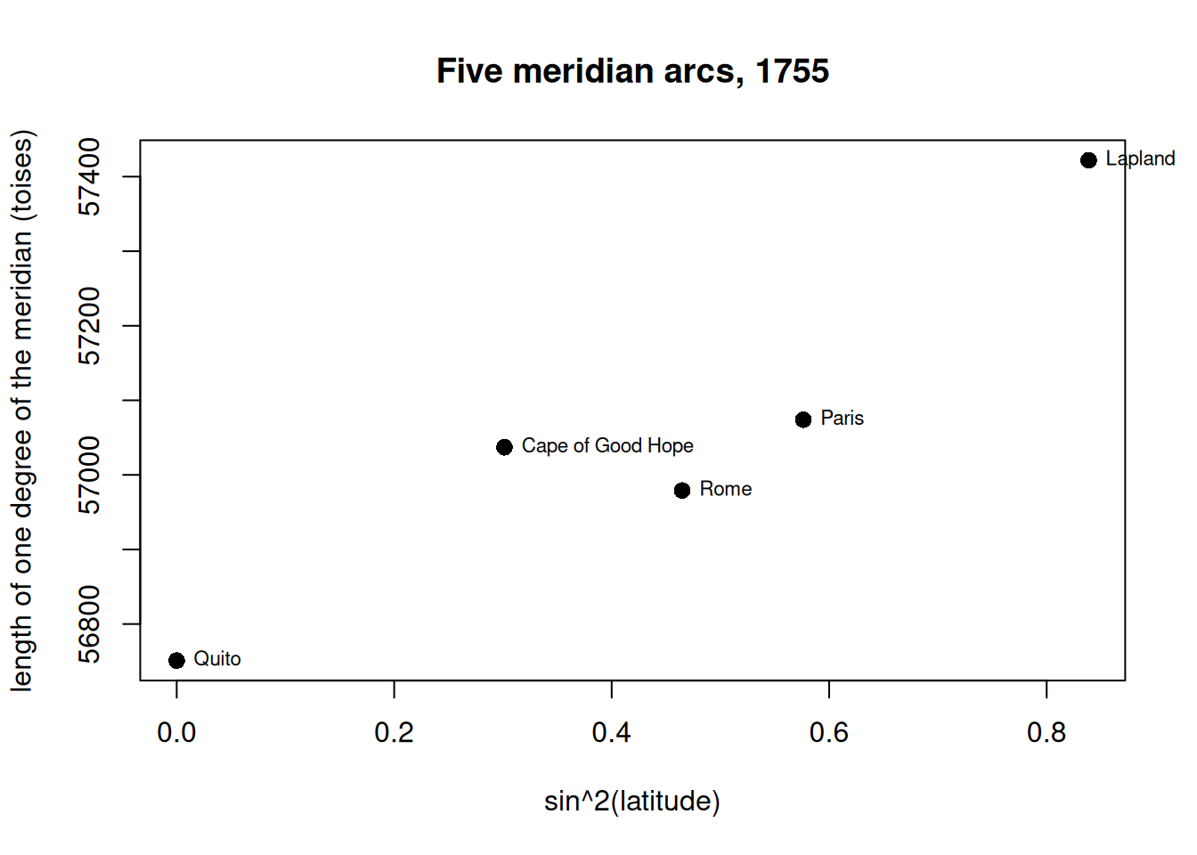

Two course-written helpers there: check_boscovich_data() validates the file the way check_mayer_data() did for Mayer’s, and add_sin2_latitude() adds the $\sin^2(\text{latitude})$ column the model needs.

Look at that plot before going on. If the Earth were a perfect sphere, these five points would sit on a flat horizontal line. They don’t — but they don’t sit on any single sloped line either, which is the whole problem.

data/boscovich_arcs.csv has five rows, one per measured arc: the place, its latitude in degrees and minutes (lat_deg, lat_min), and arc_toises, the measured length of one degree of the meridian there. A toise is an old French unit, a bit under two metres.

The equation behind Boscovich’s rows, if you’re curious

Each row is one observational equation of the form $y_i = A + B\sin^2 \theta_i$, where $y_i$ is the measured arc length, $\theta_i$ is the latitude, and $A$ and $B$ are the two unknowns. If the Earth is flattened at the poles, a degree of latitude gets longer as you go north, and it does so in proportion to $\sin^2(\text{latitude})$ — that’s the whole physical content of the model. $A$ is the arc length at the equator; $B$ says how fast it grows.

The quantity Boscovich actually reported is the ellipticity, $3A/B$ — the helpers give it as one_over_ellipticity. A value of 230 means the Earth’s polar radius is about $1/230$ shorter than its equatorial radius. A negative value means the line slopes the wrong way, i.e. an Earth stretched at the poles rather than squashed.

Every method in this problem gets judged by the same scorecard, score_line(), which reports four things about any line you hand it:

Column	What it means
`sum_abs_residuals`	total absolute error — Boscovich’s criterion
`sum_squared_residuals`	total squared error — Legendre’s criterion, from 1805
`residual_total`	the errors added up with their signs — Boscovich’s requirement that they cancel to zero
`one_over_ellipticity`	$3A/B$, the shape of the Earth this line is claiming

Part 2a — Boscovich’s method of situation

Helper functions in this part

The mathematical fact above is what makes the method computable by hand. The helper does that reduction for you:

Call	What it does for you
`boscovich_candidate_lines(arcs)`	Builds all five candidate lines and scores each one against all five arcs (points). One call, the whole method
`boscovich_residual_table(arcs)`	Lays out all 25 residuals as a table, so you can see each candidate line measured against each arc (point)
`best_line(lines, criterion = "absolute")`	Picks the winner under Boscovich’s own criterion
`plot_arc_lines(arcs, lines, main)`	Draws the arcs with any set of lines on top

Boscovich wanted the line that makes the total absolute error as small as possible, with the extra requirement that the errors cancel out to zero. That second requirement forces the line through the centre of the data, $(\bar{x}, \bar{y})$ — which kills one of the two unknowns, leaving only the slope free. And then a genuine mathematical fact about this problem takes over: the best such line always joins the centre to one of the five measured arcs. So there are only five lines to check.

That reduction is what made the method usable by hand in 1755. Run it:

candidates <- boscovich_candidate_lines(arcs)
candidates

             anchor                       method intercept_A  slope_B sum_abs_residuals sum_squared_residuals residual_total one_over_ellipticity
1             Quito             centroid + Quito    56751.00   691.39            337.52              28734.61              0               246.25
2 Cape of Good Hope centroid + Cape of Good Hope    57002.12   115.73            656.05             173218.91              0              1477.64
3              Rome              centroid + Rome    58174.85 -2572.66           3572.48            4277455.39              0               -67.84
4             Paris             centroid + Paris    56985.91   152.88            625.77             156077.45              0              1118.27
5           Lapland           centroid + Lapland    56652.18   917.93            413.91              42899.49              0               185.15

Step 1 — Read all 25 residuals

Each of the five candidate lines is scored against all five arcs, not just the one that defined it. See all 25 residuals at once:

boscovich_residual_table(arcs)

  candidate_anchored_at    Quito Cape of Good Hope   Rome   Paris Lapland
1                 Quito     0.00             77.60 -93.38  -75.38   91.16
2     Cape of Good Hope  -251.12              0.00 -76.91    5.20  322.83
3                  Rome -1423.85           -362.39   0.00  381.53 1404.71
4                 Paris  -234.91              5.01 -77.97    0.00  307.88
5               Lapland    98.82            108.13 -99.86 -107.09    0.00

Every candidate has a residual of exactly zero at its own anchor.

Answer in your hw-01.qmd: one sentence explaining why that has to be true, and why it does not mean that candidate is a good line.

Step 2 — Pick Boscovich’s answer

The candidate with the smallest total absolute error:

boscovich_answer <- best_line(candidates, criterion = "absolute")
boscovich_answer

Step 3 — Fill in the candidate table

Answer in your hw-01.qmd: fill in this table from candidates.

Candidate line (centroid + …)	Slope $B$	Sum \|resid\|	1/ellipticity
Quito
Cape of Good Hope
Rome
Paris
Lapland

Step 4 — Plot the candidates

Plot all five, then the winner alone:

plot_arc_lines(arcs, candidates, main = "Boscovich's five candidate lines")
plot_arc_lines(arcs, boscovich_answer, main = "Boscovich's answer")

Now read your one_over_ellipticity column against what people thought was real Earth’s value of about 230.

Answer in your hw-01.qmd: A negative value and a wildly large one mean different things — say what each one means.

Part 2b — The same five lines, scored by squares

Helper functions in this part

No new lines — you reuse the candidates table you already built and call best_line() on it again, switching criterion = "absolute" to criterion = "squared". That one argument is the whole of Legendre’s disagreement with Boscovich.

Fifty years later Legendre proposed a different scoreboard: minimize the sum of squared errors instead of absolute ones. He gave no argument that squares were right, only that the resulting arithmetic was tractable.

Step 1 — Rescore the same five candidates

No new lines are needed. The same five candidates get rescored:

best_line(candidates, criterion = "squared")

Answer in your hw-01.qmd: does the winner change? Report both winners and their scores.

Step 2 — Fill in the second scoreboard

Answer in your hw-01.qmd: fill in this table, next to the one from Part 2a Step 3.

Candidate	Sum \|resid\|	Sum resid²
Quito
Cape of Good Hope
Rome
Paris
Lapland

That is all Part 2b asks. Both error criteria agree about the winner here — Part 2c is where they stop agreeing, and where you work out why.

Part 2c — Every pair of arcs

Helper functions in this part

Call	What it does for you
`all_pair_lines(arcs)`	Builds and scores all ten two-arc lines in one call
`best_line(lines, criterion)`	The same helper from Parts 2a–2b, now pointed at the pairs table instead of the candidates table

Before 1750 the standard practice was simpler: pick your two best measurements and ignore the rest. Any two arcs fix $A$ and $B$ exactly. With five arcs there are only $\binom{5}{2} = 10$ such pairs, so you can just compute every one of them — no sampling needed, unlike Problem 1’s 27 equations.

pair_lines <- all_pair_lines(arcs)
pair_lines

Step 1 — The range across the ten pairs

Answer in your hw-01.qmd: the range of one_over_ellipticity across all ten pairs, and how many pairs give a negative value.

Step 2 — Do the two scoreboards rank the ten the same way?

You now have both scoreboards for the same ten lines.

Answer in your hw-01.qmd: find a pair of lines where absolute error prefers one and squared error prefers the other, and report both lines’ scores under both criteria. Then, in two or three sentences: why might that be the case?

Step 3 — Best pair under each criterion

best_line(pair_lines, criterion = "absolute")
best_line(pair_lines, criterion = "squared")

Now compare the best pair against Boscovich’s answer from Part 2a, under both criteria. You should find that the best pair beats Boscovich under one criterion and loses to him under the other.

Answer in your hw-01.qmd: all four numbers, in the table provided.

That is not the contradiction it looks like

Boscovich never allowed himself every line. His first requirement was that the errors cancel to zero, and all five of his candidates satisfy it — look at the residual_total column for them, and then at the same column for the pair lines. The winning pair does not cancel; its errors lean systematically one way. It buys its lower absolute total with a move Boscovich had ruled out, so it was never in his competition to begin with.

Part 2d — Mayer’s method on Boscovich’s five equations

Helper functions in this part

Call	What it does for you
`mayer_split_line(arcs, low_group_size)`	Sorts the arcs, cuts them into a low group and a high group at the size you name, averages each group, solves the resulting 2×2, and scores the answer — Mayer’s whole method in one call

Something that we can think of as Mayer’s rule from Problem 1 wasn’t about lunar astronomy — it was a general recipe for too-many-equations problems: sort the equations so the coefficients differ as much as possible between groups, combine within each group, and solve. Boscovich’s problem has five equations and two unknowns, so it needs two groups, not three.

Sort the arcs by $\sin^2(\text{latitude})$ and cut them into a low group and a high group. There are two sensible cuts:

split_2_3 <- mayer_split_line(arcs, low_group_size = 2)
split_3_2 <- mayer_split_line(arcs, low_group_size = 3)

rbind(split_2_3, split_3_2)

            split                          group_1                group_2 group_1_mean_sin2 group_2_mean_sin2 coefficient_spread          method intercept_A slope_B sum_abs_residuals sum_squared_residuals residual_total one_over_ellipticity
1 Mayer split 2/3        Quito + Cape of Good Hope Rome + Paris + Lapland              0.15              0.63               0.48 Mayer split 2/3    56810.28  555.50            410.26              39486.08              0               306.81
2 Mayer split 3/2 Quito + Cape of Good Hope + Rome        Paris + Lapland              0.26              0.71               0.45 Mayer split 3/2    56738.31  720.49            347.33              28308.75              0               236.25

Step 1 — Report both splits

Answer in your hw-01.qmd: each split’s two groups, its coefficient_spread (how far apart the two group averages are), and both of its residual scores.

Step 2 — Spread vs. fit

Mayer’s own stated rule says to maximize the spread between groups.

Answer in your hw-01.qmd: which split has the larger coefficient_spread? Which split actually fits better? Report the two spread values and the two sum_squared_residuals values that settle it.

Step 3 — Plot the better split

Take the split with the lower residual scores — the one you picked out in Step 2 — and draw its line against the five arcs:

better_split <- if (split_2_3$sum_abs_residuals < split_3_2$sum_abs_residuals) {
  split_2_3
} else {
  split_3_2
}

plot_arc_lines(arcs, better_split, main = "Mayer's line on the five arcs")

Answer in your hw-01.qmd: where does that line fall relative to the five measured points themselves? Mayer’s method has quietly done something neither Boscovich’s five candidates nor the ten pairs could do — say what, in one sentence.

Part 2e — Lines that miss every point

Helper functions in this part

Call	What it does for you
`score_line(arcs, intercept, slope, label)`	Scores any line you hand it. Here you hand it `lm()`’s answer, so least squares gets judged on exactly the same scorecard as every hand method
`compare_methods(...)`	Stacks scored lines from all four methods into one table

lm() is real base R functio —?lm works. Lab 01 introduced it, but we treat it as a black box for now.

Do Step 1 before you run any more code

Step 1 — Predict, before running any more code

Every method so far searched a short list you could write down: five candidate lines (Part 2a), ten pair lines (Part 2c), one line per split (Part 2d).

Answer in your hw-01.qmd: two or three sentences, in plain language, answering: is there any reason to think the best line is on one of those lists at all? If you wanted to check a line that isn’t — say, a slope halfway between two of your candidates — how would you go about deciding whether it was better, and what would stop you from doing that for every possible slope by hand in 1755?

Write your answer before running Step 2. It is graded on being a real prediction, not on being right.

Step 2 — Least squares

Now use the tool Lab 01 introduced. Treat it as a black box for now — what it does internally is a Chapter 4 question:

fit <- lm(arc_toises ~ sin2_latitude, data = arcs)
coef(fit)

least_squares <- score_line(
  arcs,
  intercept = coef(fit)[1],
  slope = coef(fit)[2],
  label = "least squares (lm)"
)
least_squares

lm() does not pick from a list. It searches every line there is and returns the one with the smallest sum_squared_residuals — the exact quantity you have been computing by hand all along.

Answer in your hw-01.qmd: one or two sentences commenting on the results you see. Where does lm()’s line land next to the ones you built by hand, and what was lm() free to do that none of those methods were?

Commit and push once both problems are done, with a message describing what’s in the commit.

Submission

Warning

Before you wrap up, make sure your Git pane is empty — everything committed and pushed.

You must also render your document to PDF and submit that PDF on Gradescope before the deadline for full credit.

To submit on Gradescope:

Access Gradescope through the menu on the STA 119FS Canvas site.
Click on the assignment, and you’ll be prompted to submit it.
Mark the pages associated with each exercise — every page of your submission should be associated with at least one question.

Unknown	Column	Report it as
\(\beta\)	`beta_arcminutes`	degrees/minutes, via `format_angle()`
\(\alpha\)	`alpha_arcminutes`	degrees/minutes, via `format_angle()`
\(\gamma = \alpha\sin\theta\)	`gamma_arcminutes`	arcminutes, as printed
\(\theta\)	`theta_degrees`	decimal degrees, as printed