Lab 04: From records to count tables

An introduction to the tidyverse

Due date

This lab is due today, by the end of class. Commit and push your lab-04.qmd and rendered PDF to your own lab repo, and submit that PDF on Gradescope.

Introduction

Today we will use two questions to practice conditional probability: Among balls in urn A, what proportion are red? And among red balls, what proportion are in urn A? The same data answer both questions, but we need a different denominator for each.

Before calculating anything, we need to organize the records. Today’s job is to make R build the tables for us. We will build a count table, calculate joint and conditional proportions by hand, and then make R reproduce those calculations. Each pipeline should tell us both what we counted and what we divided by.

Learning goals

By the end of this lab you will be able to:

read an R pipeline from top to bottom;
distinguish sorting, grouping, and summarizing;
build a count table with group_by() and summarise(), or count();
read a 2×2 count table;
calculate joint and conditional probabilities with the right denominator;
explain why filtering before or after calculating a proportion matters.

Opening activity

Laptops closed. Stay with your group and keep your card visible. We will use the 16 cards J, Q, K, and A in all four suits, with one card per person. Imagine selecting one person uniformly at random from the class. Let $A$ denote the event that their card is an Ace; similarly, $J$, $Q$, and $K$ denote Jack, Queen, and King. Write suits as $\text{Heart}$, $\text{Spade}$, and $\text{Club}$.

For each probability, decide together:

Denominator: Who is eligible to be counted? Those people stand.
Numerator: Among those standing, who satisfies the event? Those people raise their cards.
Probability: What fraction does this give?

Everyone sits back down between rounds. A different member of each rank group should explain its reasoning each time.

Start with the whole population: \[P(A),\quad P(J),\quad P(Q),\quad P(K).\] Who belongs in the denominator for each probability? Take turns having each rank group raise its cards, and report the count for each group. We have grouped by card rank and counted. How do we turn those counts into the four probabilities?
Condition on rank: \[P(\text{Heart}\mid K).\] What does the condition after the bar tell us about who should stand?
Reverse the condition, keeping the same two events: \[P(K\mid\text{Heart}).\] Who stands now? Compare the numerator and denominator with the previous round: which people are the same, and which have changed?
An “or” inside a condition: \[P(J\text{ or }Q\mid\text{Spade}).\] Who is eligible, and which eligible people satisfy at least one of those events?
An “and,” with no condition: \[P(J\text{ and Club}).\] Does the suit restrict the denominator here, or is it part of the event counted in the numerator?

Discuss: Did reversing the condition in rounds 2 and 3 change the probability? Does that mean reversed conditional probabilities must always agree? Explain using the populations you counted, then keep the question in mind for the urn activity.

From people to R

In round 1, grouping by card rank illustrates group_by(), and reporting each group’s count illustrates summarise(n = n()). Dividing those counts by the whole population gives the four rank probabilities. Choosing who stands illustrates filter(): keep only those meeting a condition. The people standing determine the denominator; raising a card identifies successes within that population.

This is an in-class discussion; there is nothing to enter in your template.

Now open your laptops — Getting your repo

Find your repo beginning with lab-04 in the statistical-history organization. Clone it in RStudio using File → New Project → Version Control → Git and its SSH address. If you have already cloned it, open that project and Pull.

Open lab-04.qmd, enter your name and group, and render once. You should also see data/urn_records.csv. Keep these instructions beside your working document. Everyone runs the code in their own repo.

Part 1 — Predict before running

The template includes eight practice records:

Record	Urn	Color
1	A	red
2	B	blue
3	A	blue
4	A	red
5	B	red
6	A	blue
7	B	blue
8	A	red

1.1 Suppose R produces one row per urn. How many rows will that table have? What if it produces one row per urn-and-color combination? Write both predictions before running anything.

Part 2 — A new way to talk to a data frame

Load the package

A package is a collection of R tools. The tidyverse is a collection of packages that work together. We will mainly use dplyr, its data manipulation package. library(tidyverse) makes these tools available in the current R session; it belongs in your document so Render loads them too. If it reports that the package is missing, tell the instructor.

library(tidyverse)

The template constructs the eight records with tibble(), a tidyverse version of a data frame. You do not need to retype them.

Read the pipe as “then”

practice |>
  filter(urn == "A")

Read this as take practice, then keep rows whose urn is A. The pipe |> passes the result on its left into the function on its right. This is another way to write filter(practice, urn == "A").

Inside these functions, write urn rather than practice$urn. Column names are unquoted; text values such as "A" need quotation marks. == asks whether values are equal. <- saves a result under a name.

2.1 Change the filter to keep blue records. How many rows remain? Did running a filter change the original practice object? Print practice to check.

Sorting is not grouping

Run these separately:

practice |>
  arrange(urn)

practice |>
  group_by(urn)

arrange() changes row order. group_by() records which rows belong together for later calculations. It does not collapse or sort the rows. Look for Groups: urn [2] above the printed grouped table.

2.2 How many rows does each result have? Which command would you use to put records from the same urn next to each other on the screen?

Now summarize

practice |>
  group_by(urn) |>
  summarise(balls = n(), .groups = "drop")

summarise() makes one summary row per group. n() counts the rows in the current group; balls is the name we chose for the output column. .groups = "drop" makes the result an ordinary, ungrouped table so a later calculation will not silently continue working within groups.

Picture the groups

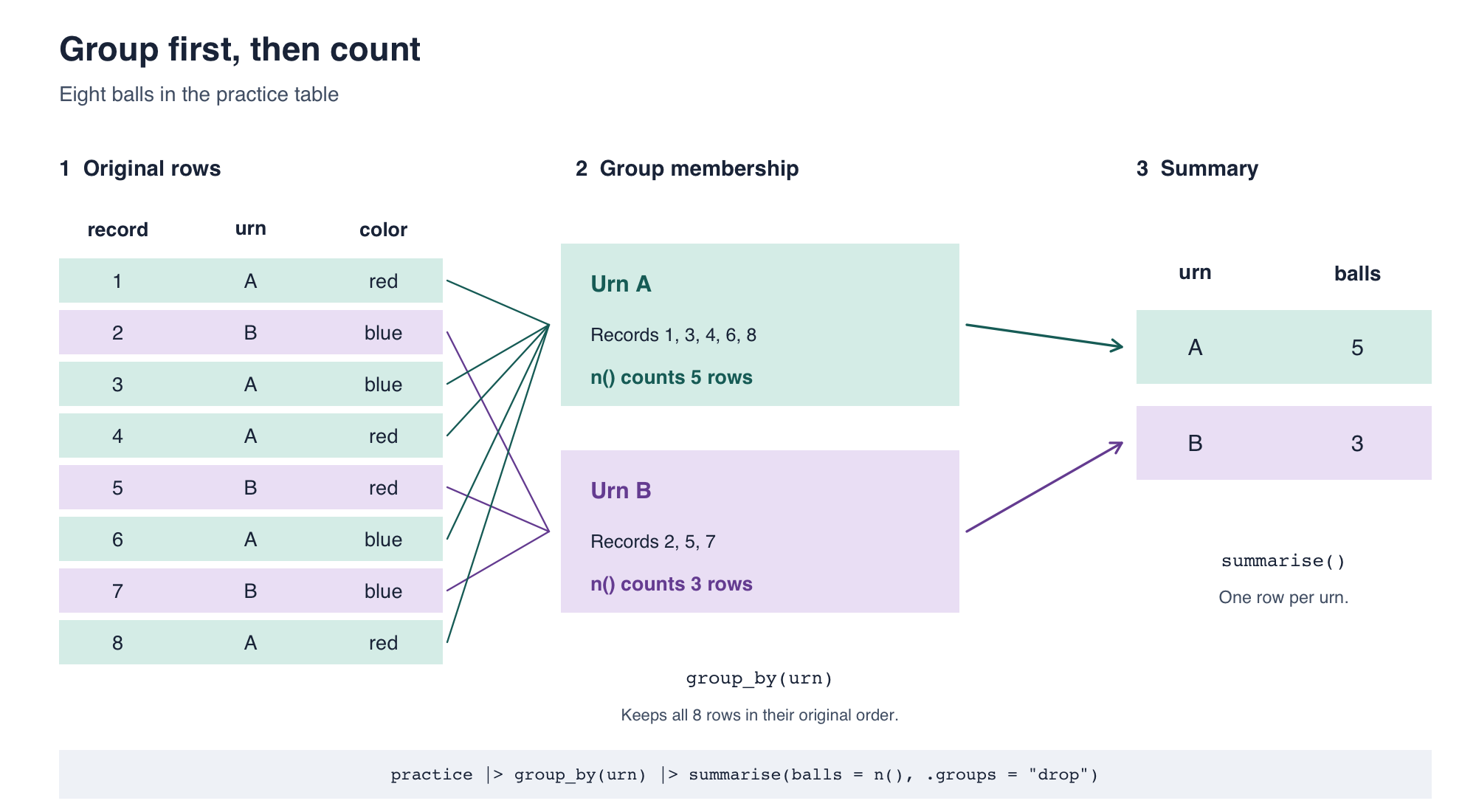
The eight practice rows retain their original order. Urn A contains records 1, 3, 4, 6, and 8; urn B contains records 2, 5, and 7. group_by(urn) identifies these groups; summarise(balls = n()) returns two rows, A with 5 balls and B with 3.

The shading marks urn membership, not ball color. group_by(urn) keeps all eight rows and tells R which belong together. Then summarise(balls = n()) counts the rows within each group and returns one row per urn. The middle boxes illustrate membership; they are not separate tables created by group_by().

2.3 Compare the number of summary rows with your first prediction. Then remove group_by(urn) and run the summary again. What does its single row represent now?

2.4 Modify the grouped version to group by both urn and color: group_by(urn, color). Compare with your second prediction. Explain what one row now represents.

Render, commit, and push

Render your document, then commit and push your work so far.

Part 3 — Build tables from a larger file

Constructed practice data

urn_records.csv is a complete inventory of 120 balls in two urns. Each row describes one distinct ball, including which urn contains it and whether it is red or blue. These 120 balls are our entire population. The urns contain different numbers of balls.

This is a fictional population created for the lab. Each ball appears exactly once. The file contains no missing values.

balls <- read_csv("data/urn_records.csv", show_col_types = FALSE)
glimpse(balls)

Column	Meaning
`record`	Unique ball identifier
`urn`	`"A"` or `"B"`, the urn containing the ball
`color`	`"red"` or `"blue"`, the ball’s color

3.1 Use group_by() and summarise() to count balls in each urn. Call the count column n. Save the resulting table as urn_totals, then print it. Check that its counts add to 120 with sum(urn_totals$n).

A shortcut for counting

For this ungrouped input, these two pipelines produce the same table:

balls |>
  group_by(urn) |>
  summarise(n = n(), .groups = "drop")

balls |>
  count(urn)

count() names the count column n automatically. It is a shortcut for a task you now know how to build from its parts.

3.2 Use count(urn, color) to save a table named urn_color. Print it and check its counts add to 120.

Always ask what a row means

In balls, one row is one ball. In urn_color, one row is an urn-and-color combination. Its n column says how many balls that combination represents. Use sum(n) to total these counts: n() would count table rows instead.

Part 4 — A 2×2 table, then pencil and paper

Use base R’s table() to display the counts with urns down the rows and colors across the columns:

table(balls$urn, balls$color)

   
    blue red
  A   32  48
  B   32   8

These are the same four counts as in urn_color, arranged in a 2×2 table. Use this table to calculate the probabilities below.

4.1 Copy the counts into your template and add the row totals, column totals, and grand total by hand. These totals will help you choose the denominators.

What probabilities are we calculating?

Imagine selecting one of the 120 balls uniformly at random: every ball across the two urns has the same chance of being selected. $P(A)$ is the probability that the selected ball is in urn A, and $P(\text{red})$ is the probability that it is red. Because our table contains every ball, its counts give these probabilities directly.

A joint probability asks whether two things are both true: $P(A \text{ and red})$. Count the balls that satisfy both conditions, but divide by all 120 balls.

A conditional probability restricts which balls we consider: $P(\text{red}\mid A)$ asks about red among A balls. Keep only urn A, then ask what fraction of those balls are red. The bar means “given.” The denominator is now the A row total, not 120.

4.2 Before using R to calculate probabilities, write a fraction for each. Write down the numerator and the denominator used for each calculation. A calculator is fine; choose the counts from your table yourself.

Question	Probability
The ball is from A	$P(A)$
The ball is red	$P(\text{red})$
The ball is from A and red	$P(A \text{ and red})$
The ball is red given it is from A	$P(\text{red}\mid A)$
The ball is from A given it is red	$P(A\mid\text{red})$

4.3 The last three fractions share the same numerator. Why do they have different denominators? Point to the relevant cell, row total, column total, or grand total in your table.

Render, commit, and push

Render your document, then commit and push before moving on.

Part 5 — Make R choose the same denominator

Joint probabilities: divide by all balls

mutate() adds a column while keeping the existing rows. Here it adds one probability for each urn-and-color combination:

joint <- urn_color |>
  mutate(probability = n / sum(n))
joint
sum(joint$probability)

Note, we are using urn_color here, not the original balls table. urn_color is ungrouped. sum(n) adds all four counts, so every row is divided by 120. The four probabilities describe mutually exclusive combinations that cover every ball, so they add to 1.

joint |>
  filter(urn == "A", color == "red")

Two conditions separated by a comma in filter() must both be true. This selects the A-and-red cell after its probability was calculated.

5.1 Compare the A-and-red result with your hand calculation. Then write a pipeline that selects the B-and-blue joint probability. State its numerator and denominator.

Conditional probabilities: filter first

To condition on A, keep A balls before counting and dividing:

colors_given_a <- balls |>
  filter(urn == "A") |>
  count(color) |>
  mutate(probability = n / sum(n))
colors_given_a

Read the steps aloud:

Keep balls from A: this sets the group we are conditioning on.
Count the colors among those retained balls.
Divide each color count by the sum of those counts: the number of A balls.

The probabilities in this table add to 1 within A. Filtering for A does not mean we already know the color: we keep both red and blue A balls so they can both contribute to the denominator.

We can also start from the summary count table:

urn_color |>
  filter(urn == "A") |>
  mutate(probability = n / sum(n))

After filtering, only the two A counts remain. sum(n) now adds those two counts. We do not call count() again on this table: its rows already contain counts of balls.

5.2 Compare both versions with your hand calculation of $P(\text{red}\mid A)$. What denominator did they use? Why must we retain the blue A balls until after division?

5.3 Reverse the condition: starting from balls, keep red balls, count urns, then add a probability column. Save this as urns_given_red. Compare its A probability with your hand calculation of $P(A\mid\text{red})$. What denominator does this pipeline use?

5.4 Starting from urn_color, calculate the color probabilities given B, then select the red row. Record the numerator and denominator. Check that the two color probabilities add to 1 before selecting red.

Part 6 — Same functions, different order

Run both pipelines. They display the same A-and-red count, but the probability columns answer different questions.

urn_color |>
  mutate(probability = n / sum(n)) |>
  filter(urn == "A", color == "red")

urn_color |>
  filter(urn == "A") |>
  mutate(probability = n / sum(n)) |>
  filter(color == "red")

6.1 For each pipeline, write down which rows are present at the moment sum(n) runs, the denominator, the resulting probability, and the question it answers. Match the results to Part 4.

6.2 A teammate filters to urn == "A", color == "red" before mutate(probability = n / sum(n)) and gets 1. Explain why. Which pipeline above should they use if they want the chance of red given A?

Part 7 — AI ethics: whose mistake is it?

You do not need an AI tool for this discussion. Start with a situation that could happen in your own group, then consider what changes when an error reaches a public audience. Both scenarios are fictional.

Round 1 — The group project

Four students complete a project together. They divide the work: one cleans the data, one analyzes it, one makes the figures, and one writes the report. Everyone’s name goes on the final submission.

The student doing the analysis uses AI to help write the code. AI use is allowed, and they tell their teammates they used it. The code runs, but it uses the wrong denominator. The student does not catch the mistake. The figures and report repeat the incorrect result. Everyone reads the final report, but nobody checks the analysis against the data. The group submits the project and learns about the error afterward.

7.1 — Who is responsible? Is responsibility limited to the student who ran the analysis, shared equally, or shared in different ways? Decide as a group and explain. Does dividing up the work also divide responsibility for the finished project? Distinguish who should have caught the mistake, who should help fix it, and who should lose credit, if anyone. Those do not have to be the same answer.

Follow-up: Would your answer change if that student had written the same incorrect code without AI? What if a teammate had specifically asked whether the denominator had been checked and been told “yes”?

Round 2 — Now it is published

Imagine that a student journalist writes an article for The Chronicle about teaching evaluations at Duke. They use AI to analyze the ratings and turn the results into a chart. An editor reviews the article and approves publication, but nobody checks the rating scale against the original survey.

In this fictional story, Kat’s ratings are all 5 out of 5, naturally. The AI assumes the scale runs from 0 to 10 and labels her average as “50% of the maximum rating.” The article presents this as evidence of poor teaching. Readers share the chart, and students decide not to sign up for Kat’s classes.

The error is discovered. The article is corrected, with a note explaining that the original analysis used the wrong scale. But screenshots of the original chart are already circulating.

7.2 — Who owns the published claim? What responsibility belongs to the journalist, the editor, the publication, and the AI provider? Do not assume all four have the same role or the same ability to check this particular analysis. Does saying “the AI made the mistake” settle anyone’s responsibility? Name one concrete check that should have happened before publication, and who should have performed it.

7.3 — Can a correction undo the harm? Can the publication be sure that everyone who saw the original will see the correction? Is editing the article enough? Propose two additional actions, say who should take them, and explain what harm might remain even afterward. If the editors instead retract the article entirely, does that solve the problem?

Spend two minutes reading, five discussing both rounds, and three writing brief answers. You may record a disagreement within your group rather than pretending to agree. Finish by naming one review habit you would adopt for your own next group project.

Wrap-up

Render, commit, push, and submit

Render your document and inspect the PDF. Check that you have attempted each required code task, completed the count table and hand calculations, compared the two pipeline orders, and written the ethics recommendation. Errors with an explanation still count as attempts. Commit and push the .qmd and PDF, then upload that PDF to Gradescope. Keep a checkpoint commit after the hand calculations and a final commit after the discussion. If you used AI elsewhere in the lab, keep commits before and after that use.

Exit ticket (on paper, with your name):

Muddiest point.
One thing you learned today.
Favorite subject in High School.

References

The progression from inspecting grouped data to summarizing it was inspired by STA 199, Fall 2025, Lab 2. The urn examples and exercises here were written for STA 119FS. Function references: group_by(), summarise(), and count().

Question	Probability
The ball is from A	\(P(A)\)
The ball is red	\(P(\text{red})\)
The ball is from A and red	\(P(A \text{ and red})\)
The ball is red given it is from A	\(P(\text{red}\mid A)\)
The ball is from A given it is red	\(P(A\mid\text{red})\)