p0_six <-NA # replace with your code
p0_sixLab 03: How many trials are enough?
ImportantDue date
This lab is due today, by the end of class. To be considered on time:
lab-03.qmdcommitted and pushed to your GitHub repo before the exit ticket- That same document, rendered to PDF, submitted on Gradescope
Introduction
Consider the following experiment: roll a die four times, and win if at least one six turns up. Today you will build this experiment in R, and then ask a question: how many times would you have to play before the dice told you anything?
Learning goals
By the end of this lab you will be able to…
- count a probability through its complement.
- write a simulator for an event whose one trial contains several actions.
- understand the difference between \(N\) (the trials in one experiment) and \(B\) (repetitions of the whole experiment).
- state what passing a frequency check does and does not establish about a die.
Getting your repo
1 · Find the repo. The statistical-history organization, the repo whose name starts with lab-03.
2 · Clone it. RStudio: File → New Project → Version Control → Git, paste the SSH address, Create Project. You should see lab-03.qmd and lab-03-helpers.R.
3 · Names in the YAML, then Render once before you change anything.
TipPull first. Yes, again.
It is your own repo and nobody else has touched it. Pull anyway — the habit is the point, and the one week you skip it is the week it matters.
Part 1 — Make a guess.
Before anyone opens a laptop
Write your guess. No computing and no looking anything up. The only wrong answer is a blank one.
Guess. Someone hands you a die and says it is fair. You are allowed to roll it in blocks of four and count how often at least one six turns up. How many blocks would you want before you would be willing to say the die looks honest? One number.
Part 2 — Count it first
Goal: get the honest probability by counting.
One trial is four rolls of a fair die, and a trial is a success if at least one of the four is a six.
The direct count is a nuisance: you would have to add up the cases of exactly one six, exactly two, exactly three, and exactly four, and it is very easy to double-count. Count the complement instead — the trials with no six at all.
Four rolls give \(6^4 = 1296\) equally likely ordered outcomes. A trial with no six uses only the other five faces, so there are \(5^4 = 625\) of those. Everything else has at least one six:
\[p_0 = 1 - \frac{5^4}{6^4} = 1 - \frac{625}{1296} = \frac{671}{1296}.\]
Fill in a code chunk in your template to calculate and save this probability.
TipStop and answer — Part 2
- Why is this not \(1/6\)? And why is it not \(4 \times 1/6 = 2/3\)? Say what each of those two wrong answers is actually the probability of.
- Suppose the game were six rolls instead of four. Write the probability down the same way and compute it. Which direction did it move, and does the complement trick still work?
Part 3 — Build the mechanism
options(digits = 7)

source("lab-03-helpers.R")
WarningThree of today’s functions are not R
check_indicators(), simulate_grid() and plot_certainty() were written for this course. They live in lab-03-helpers.R, which is the file you just sourced. Open the file if you want to see what each function does in more details; there is an index at the top and comments above each function.
| Call | What it does for you | First used |
|---|---|---|
check_indicators(x, N) |
Confirms a vector is exactly N zeros and ones. Prints nothing when happy |
Part 3 |
simulate_grid(N_values, p0, epsilon, certainty_odds, B, model_p) |
Runs a whole study at each N you name and stacks the results into one table |
Part 5 |
plot_certainty(results, certainty_odds) |
Plots one of those tables, with the target marked | Part 6 |
There is a fourth, summarize_experiments(), which turns a pile of success counts into one row of that table. You never call it — simulate_grid() calls it for you, once per N. It is in the file if you are curious.
Everything else today is real base R and is documented, so ?sample works: sample(), rbinom(), numeric(), seq_len(), any(), as.integer(), mean(), table(), data.frame() and set.seed().
Goal: a function that plays the game N times and reports, for each of those N trials, whether it was a success.
play_six <- function(N) {
  outcomes <- numeric(N)

  for (i in seq_len(N)) {
    rolls <- sample(1:6, size = 4, replace = TRUE)
    outcomes[i] <- as.integer(any(rolls == 6))
  }

  outcomes
}
Line by line:
| The code | What it does |
|---|---|
numeric(N) |
Makes room for N results before the loop starts |
seq_len(N) |
The trial numbers, 1 through N |
sample(1:6, size = 4, replace = TRUE) |
Rolls the die four times — one whole trial |
replace = TRUE |
Rolling a 3 does not remove the 3 from the die |
any(rolls == 6) |
TRUE if at least one of the four was a six |
as.integer() |
Turns TRUE/FALSE into 1/0 so it can be averaged |
set.seed(20260918)

small_run <- play_six(20)
check_indicators(small_run, 20)
table(small_run)
small_run
0 1
9 11 large_run <- play_six(50000)
check_indicators(large_run, 50000)
data.frame(
calculated_p0 = p0_six,
simulated_rate = mean(large_run),
difference = mean(large_run) - p0_six
) calculated_p0 simulated_rate difference
1 0.5177469 0.51528 -0.002466914check_indicators() prints nothing when it is happy. That is the intended output. It stops with an error if the vector is the wrong length or contains something other than 0 and 1 — and note what it does not check: it has no idea whether you rolled a six-sided die or a twenty-sided one.
Note
set.seed() — what it does, and where it must not go
R’s randomness is not really random; it is a long fixed sequence, and set.seed(n) says start reading at position n. Two people who set the same seed get the same rolls, which is what makes a simulation reproducible — and why every chunk today carries one.
Set it before a study, never inside a function. If set.seed() sat inside play_six(), every trial would restart the sequence at the same place and all N trials would come out identical. The seed above is in the chunk, outside the function, which is exactly right.
TipStop and answer — Part 3
- Which line makes a new trial start afresh (runs a new experiment of rolling a die 4 times)? Point at it.
- Suppose instead you rolled the die 200 times in one long sequence and slid a four-roll window along it — rolls 1–4, then 2–5, then 3–6. That also gives you “trials.” Why are those not independent?
- What does
calculated_p0tell us and what doessimulated_ratetell us? How are the two different?
Part 4 — What we are actually going to do
Goal: before choosing any numbers, get the whole procedure straight. Everything after this is just running it.
Part 3 gave you one experiment, play_six(N), that plays the game N times and mean() turns successes of each game into a single proportion. The question this lab exists to answer is what should N be and what to do with that number when someone hands you a die and says it is fair.
Here is the procedure, start to finish.
· The claim. Someone says the die is fair. If they are right, one trial — four rolls, looking for at least one six — succeeds with chance \(p_0 = 0.5177\). That is the number you counted in Part 2, and it is the only thing the claim buys us.
· What “chance** \(0.5177\)” actually promises. Not that an experiment with a fixed N will give you \(0.5177\). It promises that as you keep playing, the proportion of trials that succeed settles near \(0.5177\). You already saw this in Part 3: 50,000 trials gave 0.5153**, close to the counted value but not equal to it.
· One experiment gives one number. Play \(N\) trials, count \(m\) successes, and you have \(\widehat p = m/N\). Run it again and you get a different one — different rolls, different count. That is the whole difficulty. You are trying to judge a fixed die using a number that moves.
· So we allow a tolerance. How far may \(\widehat p\) sit from \(p_0\) before we object? Call that distance \(\epsilon\). The interval
\[[\,p_0 - \epsilon,\; p_0 + \epsilon\,]\]
is the acceptance band, and one experiment passes the check if its \(\widehat p\) lands inside it. That phrase — passes the check — is what the rest of the lab is about.
· And we set a standard. Because \(\widehat p\) moves, an honest die will sometimes miss the band by bad luck. We want that to be rare. So we demand: an honest die must pass at least \(c/(c+1)\) of the time.
· What we are actually looking for. Every number here is computed assuming the die is fair — \(p_0 = 0.5177\) is what a fair die gives, and the band is drawn around it. So the goal, stated as something we can aim at:
Find an \(N\) big enough that a fair die almost never lands outside the band.
Turn that around and you have the reason anyone would want such an \(N\). If at that size a fair die falls outside only once in a hundred tries, then someone who runs a single experiment and lands outside has just seen something that rarely happens to fair dice. That is worth flagging. It is a result you would not shrug at.
That is the whole use of \(N\): the experiment size at which landing outside the band stops being ordinary and starts being worth a second look. Too small an \(N\) and honest dice fall outside constantly, so the flag means nothing.
We find it by simulation, because there we set the truth ourselves. Play the whole experiment \(B\) times from a die we have deliberately made fair, and count how many passed. That proportion estimates
\[q_N = P\big(\,|\widehat p - p_0| \le \epsilon\,\big),\]
and we want \(q_N \ge c/(c+1)\) — equivalently, the chance of landing outside is at most \(1/(c+1)\), which for \(c = 99\) is one in a hundred.
WarningA threshold for surprise, not a verdict
Landing outside the band is unlikely if the die is fair. That is a statement about fair dice. It is not the same as “the die is probably unfair,” and the two come apart in a way that matters. The debrief pulls them apart.
For now: you are building a threshold for surprise, not a verdict.
ImportantTwo numbers, two jobs — this is the distinction the whole lab turns on
| What it is | What it controls | |
|---|---|---|
| \(N\) | trials inside one experiment | how much \(\widehat p\) bounces around. Bigger \(N\), steadier \(\widehat p\) |
| \(B\) | how many whole experiments we simulate | how precisely we know \(q_N\). Bigger \(B\), sharper estimate |
\(N\) is a fact about the study someone would actually run. \(B\) exists only because we are using a simulation to determine \(N\).
Now the two choices
Neither has a correct answer. Both are ours to make, and the debrief comes back to how much they were doing.
| Choice | What it means | Ours in this Lab |
|---|---|---|
| Tolerance \(\epsilon\) | How far \(\widehat p\) may sit from \(p_0\) and still pass | \(p_0/5\) — a 20% relative discrepancy |
| Certainty odds \(c:1\) | How often an honest die must pass | \(99:1\), i.e. probability \(99/100\) |
epsilon_six <- p0_six / 5
c_odds_six <- 99
target_six <- c_odds_six / (c_odds_six + 1)

data.frame(
  p0 = p0_six,
  epsilon = epsilon_six,
  band_lower = p0_six - epsilon_six,
  band_upper = p0_six + epsilon_six,
  certainty_odds = c_odds_six,
  target_probability = target_six
)
p0 epsilon band_lower band_upper certainty_odds target_probability
1 0.5177469 0.1035494 0.4141975 0.6212963 99 0.99band_lower and band_upper are the two ends of the acceptance band. An experiment passes if its \(\widehat p\) falls between them, endpoints included.
ImportantMaking \(\epsilon\) a fraction of \(p_0\) is itself a decision
We could have picked a flat number — 0.02, say, the way Bernoulli did for his urn. Writing it as \(p_0/5\) instead means the tolerance scales with the event: a common event gets a wide band and a rare one gets a narrow band.
That choice is doing more work than it looks like, and HW 02 makes you feel it. Hold on to this one; the debrief comes back to it.
TipStop and answer — Part 4
- Our band is \([0.414, 0.621]\) — more than a fifth of the whole probability scale wide. Name a use for this check where that width is fine, and one where it plainly is not.
- A die is loaded so that a six comes up with chance \(1/5\) instead of \(1/6\). That makes this event’s probability \(1 - (4/5)^4\). Add a code chunk to calculate this value. Does this value fall inside the band we chose?
Part 5 — Run it once, for a fixed \(N\).
Goal: see what the helper’s table actually reports, at a large \(N\).
Part 3 ran 50,000 trials. Let us keep that size, and run the honest-model study described above: simulate \(B = 10{,}000\) whole experiments of 50,000 trials each, and count how many pass.
set.seed(61000)

six_fixed <- simulate_grid(
  N_values = 50000,
  p0 = p0_six,
  epsilon = epsilon_six,
  certainty_odds = c_odds_six,
  B = 10000
)

six_fixed
N B inside outside q_hat odds_hat lower95 upper95 assessment
1 50000 10000 10000 0 1 NA 0.9996312 1 meetsAll 10,000 experiments passed. At this size \(\widehat p\) has essentially nowhere to go, so that is no surprise.
| Column | What it is claiming | Here |
|---|---|---|
inside, outside |
How many of the \(B\) experiments passed and failed. They add to \(B\) | 10,000 and 0 |
q_hat |
inside / B — the estimated chance that a whole experiment passes |
1.0000 |
odds_hat |
inside / outside. NA means no failures were seen, not that the odds are infinite |
NA |
lower95, upper95 |
How much to trust q_hat, given how many experiments you ran — see below |
0.99963 to 1 |
assessment |
Those two, compared against the \(99/100\) target | meets |
How to read the simulation uncertainty
The helpers report lower95 and upper95, a 95% Monte Carlo interval for \(q_N\). You do not need to understand how it is built and what it means beyond that it describes the precision of your simulation estimate, and it is a separate thing from your chosen \(99:1\) requirement.
assessment |
Interpretation at this tested \(N\) |
|---|---|
meets |
The whole interval is at or above \(c/(c+1)\) |
below |
The whole interval is below \(c/(c+1)\) |
unresolved |
The interval straddles the target — this simulation is not precise enough to decide |
If assessment says unresolved, it means \(B\) is not high enough to make a decision about \(q_N\). Not that the die failed, and not that this \(N\) is wrong — only that this many experiments cannot tell which side of the target the truth is on. The fix is more experiments, not more trials.
TipStop and answer — Part 5
q_hatcame back as exactly 1. How many of the 10,000 experiments had their \(\widehat p\) land inside the band? And what does that have to do withodds_hatprintingNA?- Imagine you have a slider that controls \(\epsilon\), keeping everything else the same. Suppose you drag it towards zero, thus, making the band narrower around the same \(p_0\). Would
q_hatgo up or down as the slider for epsilon gets closer to zero?
Part 6 — Can we get away with less?
Goal: \(N = 50{,}000\) works, but it is 200,000 individual rolls and nobody is doing that at a table. We will now test a variety of different values of \(N\) and try to find the smallest experiment size that still clears the standard.
NoteWhat we are really searching for
Remember, we are trying to find \(N\) such that if we run the experiment and calculate \(\hat p\), it would land within \(\epsilon\) of the truth \(p_0\) with probability \(\frac{c}{c+1}\).
We start by checking a wide variety of values of \(N\) and assess them with \(B=10,000\) repetitions.
set.seed(61001)

six_N <- c(25, 50, 100, 150, 200, 250, 300, 400, 500, 750, 1000)

six_pilot <- simulate_grid(
  N_values = six_N,
  p0 = p0_six,
  epsilon = epsilon_six,
  certainty_odds = c_odds_six,
  B = 10000
)

six_pilot
N B inside outside q_hat odds_hat lower95 upper95 assessment
1 25 10000 6846 3154 0.6846 2.170577 0.6753898 0.6937026 below
2 50 10000 8813 1187 0.8813 7.424600 0.8747995 0.8875775 below
3 100 10000 9657 343 0.9657 28.154519 0.9619446 0.9691809 below
4 150 10000 9889 111 0.9889 89.090090 0.9866479 0.9908601 unresolved
5 200 10000 9968 32 0.9968 311.500000 0.9954855 0.9978102 meets
6 250 10000 9987 13 0.9987 768.230769 0.9977780 0.9993076 meets
7 300 10000 9998 2 0.9998 4999.000000 0.9992777 0.9999758 meets
8 400 10000 10000 0 1.0000 NA 0.9996312 1.0000000 meets
9 500 10000 10000 0 1.0000 NA 0.9996312 1.0000000 meets
10 750 10000 10000 0 1.0000 NA 0.9996312 1.0000000 meets
11 1000 10000 10000 0 1.0000 NA 0.9996312 1.0000000 meetsWe now plot estimated \(\hat q_N\) for each \(N\) we tested. The dashed horizontal line corresponds to our goal of \(q_N = 0.99\).
plot_certainty(six_pilot, certainty_odds = c_odds_six)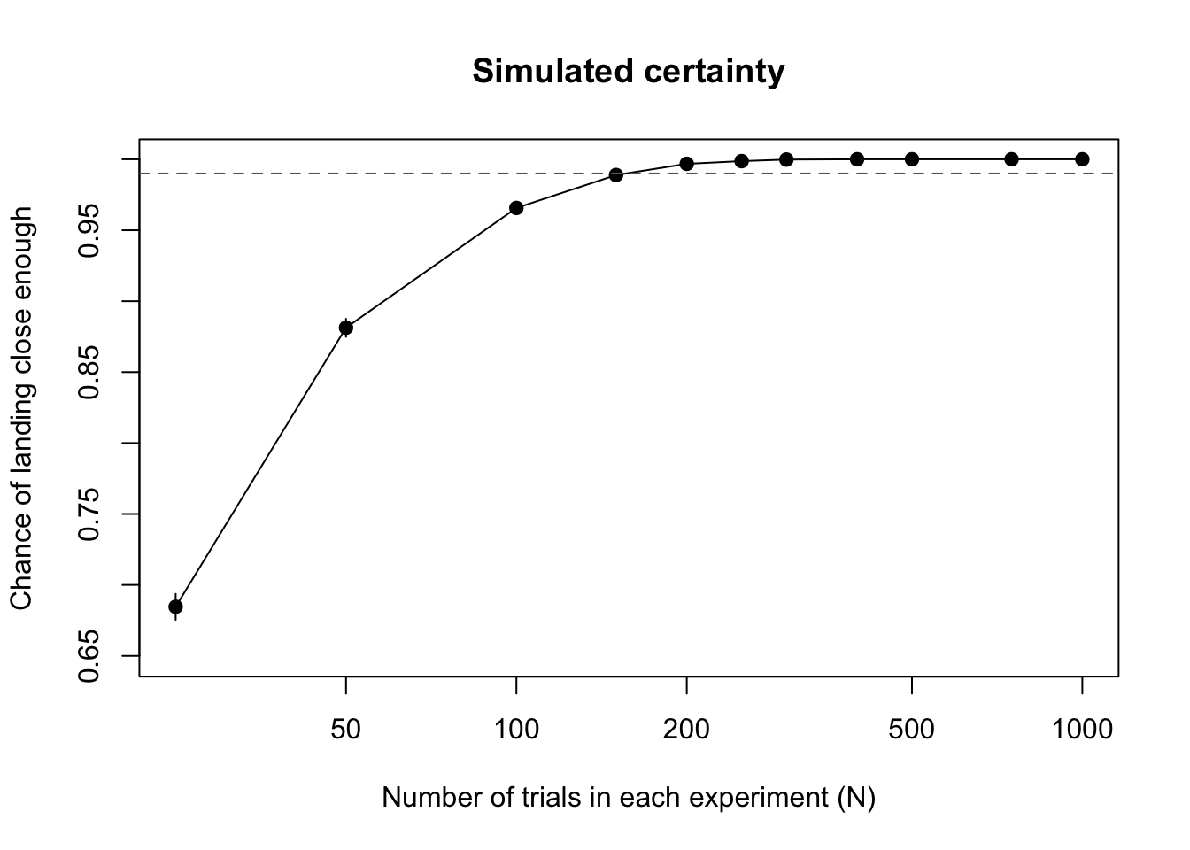
Read down the assessment column, not the q_hat column. Three rows matter:
| \(N\) | q_hat |
assessment |
What it tells you |
|---|---|---|---|
| 100 | 0.9657 | below |
Too small. The whole interval is under 0.99 |
| 150 | 0.9889 | unresolved |
Above 0.99 as a point estimate, and still not callable — the interval crosses the line |
| 200 | 0.9968 | meets |
Clears it, interval and all |
So the transition is somewhere between 100 and 200. We have looked at 150 but did not use sufficiently large \(B\) to draw conclusions. Everything from 250 up also passes, but those are more expensive and tell us nothing new. Zoom in on the window that is actually in doubt.
set.seed(61002)

six_refined_N <- c(105, 115, 125, 135, 145, 155, 165, 175, 185, 195)

six_refined <- simulate_grid(
  N_values = six_refined_N,
  p0 = p0_six,
  epsilon = epsilon_six,
  certainty_odds = c_odds_six,
  B = 10000
)

six_refined
N B inside outside q_hat odds_hat lower95 upper95 assessment
1 105 10000 9654 346 0.9654 27.90173 0.9616297 0.9688960 below
2 115 10000 9754 246 0.9754 39.65041 0.9721719 0.9783470 below
3 125 10000 9790 210 0.9790 46.61905 0.9759962 0.9817201 below
4 135 10000 9840 160 0.9840 61.50000 0.9813449 0.9863675 below
5 145 10000 9868 132 0.9868 74.75758 0.9843657 0.9889443 below
6 155 10000 9884 116 0.9884 85.20690 0.9861030 0.9904055 unresolved
7 165 10000 9911 89 0.9911 111.35955 0.9890590 0.9928466 unresolved
8 175 10000 9945 55 0.9945 180.81818 0.9928469 0.9958540 meets
9 185 10000 9949 51 0.9949 195.07843 0.9932998 0.9962004 meets
10 195 10000 9967 33 0.9967 302.03030 0.9953687 0.9977274 meets145 and lower are below. 155 and 165 are still unresolved; 175 and up all read meets. Notice what that does and does not establish. It says 175 passed at this \(B\), on this seed. It does not say 174 fails, and it does not say 175 is the smallest possible — we tested ten numbers out of a hundred.
TipStop and answer — Part 6
- In the pilot, between which two values of \(N\) does
assessmentstop sayingbelow? - 155 comes back
unresolvedat the same \(B\) as before. What one change would settle if \(155\) is large enough? - \(N\) and \(B\) both make things “more accurate,” but not the same thing. One of them sharpens our estimate of \(\widehat p\); the other sharpens our estimate of \(P(\widehat p \text{ lands in the band})\). Which does which ?
Part 7 — Confirm it
Goal: one fresh study, at a new seed and ten times the experiments, on the values the search could not settle.
Which values are worth re-testing, and why \(B\) jumps
The refinement left 155 and 165 unresolved and put the first meets at 175. Those three are the ones to confirm — and notice it is not the below rows that are worth re-running. 105 through 145 came back with their whole intervals under the target; running them again at ten times the cost would only say below in more decimal places.
The undecided ones are different. unresolved means the study could not tell which side of the target the truth was on. Look harder and it might come back meets — which would hand you a smaller, cheaper answer than 175. That is the entire reason to spend the extra experiments.
And \(B\) goes from 10,000 to 100,000 because our target is 0.99: we are trying to measure a failure rate of about one in a hundred, and 10,000 experiments expect only about 100 failures. Ten times the experiments, ten times the resolution — on \(q_N\), not on the die.
ImportantFix your values before you run this
A confirmation is only worth something if you chose what to confirm beforehand. Write 155, 165 and 175 down. Then run the chunk once.
Rerunning with new seeds until something passes is not a confirmation — it is a search wearing a confirmation’s clothes, and it makes the number meaningless.
set.seed(61003)

six_confirm_N <- c(155, 165, 175)

six_confirmation <- simulate_grid(
  N_values = six_confirm_N,
  p0 = p0_six,
  epsilon = epsilon_six,
  certainty_odds = c_odds_six,
  B = 100000
)

six_confirmation
N B inside outside q_hat odds_hat lower95 upper95 assessment
1 155 100000 99020 980 0.99020 101.0408 0.9895700 0.9908013 unresolved
2 165 100000 99203 797 0.99203 124.4705 0.9914594 0.9925718 meets
3 175 100000 99378 622 0.99378 159.7717 0.9932731 0.9942579 meets165 resolved. At \(B = 10{,}000\) it was undecided; at \(B = 100{,}000\) it reads meets, at \(\widehat q = 0.99203\) with the whole interval above the target. So the answer improves from 175 to 165 — the extra experiments bought a smaller \(N\), which is exactly what we hoped for and why the smaller values were worth testing at all.
155 did not resolve. It is still unresolved at ten times the effort, sitting at \(0.99020\) with its interval straddling 0.99.
WarningNot every
unresolved is a shortage of experiments
165 was undecided because \(B\) was too small — look harder and it settles. 155 is a different animal. Its true pass rate sits almost exactly on 0.99, so no affordable number of experiments will ever put it cleanly on one side. More \(B\) would not help.
That is a real and reportable result, not a failure. The honest statement is: 165 is the smallest tested size we can support; 155 we cannot resolve, and would need far more than 100,000 experiments to try.
TipStop and answer — Part 7
- The refinement said 175 and the confirmation says 165. Which is the better answer, and what did the extra experiments actually buy you?
- 105 through 145 all came back
belowin the refinement, and we did not re-run them here. Why not? What would testing them again have told you?
Part 8 — Debrief
Back together as a room.
One — you found \(N\). Now what?
ImportantThe question Part 4 left open
Everything today assumed the die is fair. So the study cannot tell you a die is fair — it only found how big an experiment a fair die needs.
Now hand that \(N\) to someone holding a real die they know nothing about. They roll \(N\) trials and get one \(\widehat p\).
Suppose their \(\widehat p\) lands outside the band. You built the check so that a fair die stays inside 99 times out of 100. So what has just happened, and what should they think?
Say it carefully — and then say what they should think if it lands inside instead.
Two — which way does \(N\) move?
Everything today held \(\epsilon\), \(c\) and \(p_0\) fixed and hunted for \(N\). Now turn the handle the other way: change one of those three and ask what \(N\) would have to do to keep the same standard.
Say bigger, smaller, or no change — and why.
(a) We make \(\epsilon\) smaller — a narrower band, everything else the same.
(b) We make \(c\) larger — say \(999:1\) instead of \(99:1\).
Part 9 — AI slot: the Decision Audit
Open a fresh chat and give it exactly this, and nothing else:
I roll a die 7 times. What is the probability I get at least one six?
That is Part 2’s question with a 7 in place of the 4, so you can check its arithmetic yourself — and it will almost certainly get the arithmetic right. The answer is not what we are auditing.
Your deliverable is a list of everything it had to decide before it could answer at all, none of which you told it.
You can start here.
| It had to assume something about… | Ask yourself |
|---|---|
| How many sides the die has | You never said six. Did it say it was assuming six, or just use it? |
| Whether the die is fair | Did it ask? Did it flag it? |
| Whether the rolls are independent | How does it combine probabilities from different rolls |
| What you wanted it for | A homework answer, a bet, a dice-tower audit? The number is the same; what you should do with it is not |
Hand in a list of things it had to decide on and which of those it told you about.
Exit ticket
- Muddiest point?
- One thing you’ve learned today.
- What is your home town?
Make sure your name is on it as this is how attendance is taken.